Attention 메커니즘 완벽 구현: Bahdanau vs Luong, 무엇이 다른가?

TL;DR: Attention은 디코더가 인코더의 모든 hidden state를 "참조"할 수 있게 합니다. Bahdanau는 additive, Luong은 multiplicative 방식입니다. 실제로는 Luong이 더 빠르고 성능도 비슷합니다.

1. 왜 Attention이 필요한가?

1.1 Seq2Seq의 병목: Context Vector

기본 Seq2Seq의 구조를 다시 살펴봅시다:

인코더: [x₁, x₂, ..., xₙ] → h_n (context vector)
디코더: h_n → [y₁, y₂, ..., yₘ]

문제: 아무리 긴 문장도 하나의 고정 크기 벡터로 압축됩니다.

$c = h_n^{enc} \in \mathbb{R}^d$

이것은 마치 1000페이지 책의 내용을 140자 트윗으로 요약하는 것과 같습니다.

1.2 긴 문장에서의 성능 저하

Cho et al. (2014)의 실험 결과:

문장 길이	BLEU Score
10 이하	25.3
20	22.1
30	18.7
40	14.2
50 이상	10.5

문장이 길어질수록 성능이 급격히 하락합니다.

1.3 Attention의 핵심 아이디어

"번역할 때 원문의 특정 부분에 '주목'한다"

사람이 번역할 때를 생각해보세요:

"I love machine learning" → "나는 기계 학습을 사랑한다"
"love" → "사랑한다"를 번역할 때, "love"에 집중
"machine learning" → "기계 학습"을 번역할 때, 해당 부분에 집중

Attention은 이 직관을 수학적으로 구현합니다.

2. Attention의 수학적 기초

2.1 핵심 수식

Attention의 핵심은 가중 평균입니다:

$c_t = \sum_{i=1}^{n} \alpha_{ti} \cdot h_i^{enc}$

여기서:

$c_t$ : 시점 $t$ 에서의 context vector (동적!)
$\alpha_{ti}$ : 시점 $t$ 에서 인코더 $i$ 번째 hidden state에 대한 attention weight
$h_i^{enc}$ : 인코더의 $i$ 번째 hidden state

핵심 포인트: context vector가 각 디코딩 스텝마다 다르게 계산됩니다!

2.2 Attention Weight 계산

$\alpha_{ti} = \frac{\exp(e_{ti})}{\sum_{j=1}^{n} \exp(e_{tj})}$

여기서 $e_{ti}$ 는 alignment score (또는 energy)입니다.

Softmax를 통해:

모든 weight의 합이 1
각 weight가 0~1 사이
"확률 분포"로 해석 가능

2.3 Score Function: Bahdanau vs Luong

여기서 두 접근법이 갈립니다. score를 어떻게 계산할 것인가?

3. Bahdanau Attention (Additive)

3.1 핵심 아이디어

Bahdanau et al. (2015)의 접근:

"디코더의 이전 hidden state와 인코더의 각 hidden state를 concat한 후 MLP로 score 계산"

3.2 수학적 정의

$e_{ti} = v^T \tanh(W_s h_{t-1}^{dec} + W_h h_i^{enc})$

여기서:

$h_{t-1}^{dec}$ : 디코더의 이전 hidden state
$h_i^{enc}$ : 인코더의 $i$ 번째 hidden state
$W_s, W_h$ : 학습 가능한 weight matrices
$v$ : 학습 가능한 weight vector

3.3 전체 디코딩 과정

1. 인코더 실행: h₁, h₂, ..., hₙ (모든 hidden states 저장)
2. 각 디코딩 스텝 t에서:
a. score 계산: e_ti = v^T tanh(W_s h_{t-1} + W_h h_i) for all i
b. attention weight: α_ti = softmax(e_ti)
c. context vector: c_t = Σ α_ti * h_i
d. 디코더 입력: [y_{t-1}; c_t] (concat)
e. 디코더 출력: h_t, y_t

3.4 PyTorch 구현

python

class BahdanauAttention(nn.Module):
    def __init__(self, encoder_dim, decoder_dim, attention_dim):
        super().__init__()
        self.encoder_att = nn.Linear(encoder_dim, attention_dim, bias=False)
        self.decoder_att = nn.Linear(decoder_dim, attention_dim, bias=False)
        self.v = nn.Linear(attention_dim, 1, bias=False)

    def forward(self, encoder_outputs, decoder_hidden):
        """
        encoder_outputs: (batch, src_len, encoder_dim)
        decoder_hidden: (batch, decoder_dim)
        """
        # decoder_hidden을 src_len만큼 복제
        decoder_hidden = decoder_hidden.unsqueeze(1)  # (batch, 1, decoder_dim)

        # Score 계산
        encoder_proj = self.encoder_att(encoder_outputs)  # (batch, src_len, attention_dim)
        decoder_proj = self.decoder_att(decoder_hidden)   # (batch, 1, attention_dim)

        energy = torch.tanh(encoder_proj + decoder_proj)  # (batch, src_len, attention_dim)
        scores = self.v(energy).squeeze(-1)               # (batch, src_len)

        # Attention weights
        attn_weights = F.softmax(scores, dim=1)           # (batch, src_len)

        # Context vector
        context = torch.bmm(attn_weights.unsqueeze(1), encoder_outputs)
        context = context.squeeze(1)                       # (batch, encoder_dim)

        return context, attn_weights

3.5 Bahdanau의 특징

장점:

이론적으로 더 표현력이 좋음 (비선형 변환 포함)
원 논문에서 검증됨

단점:

계산량이 많음 (MLP 연산)
구현이 복잡

4. Luong Attention (Multiplicative)

4.1 핵심 아이디어

Luong et al. (2015)의 접근:

"현재 디코더 hidden state와 인코더 hidden state의 내적으로 score 계산"

4.2 세 가지 Score Function

Luong은 세 가지 score function을 제안했습니다:

1. Dot Product:

$e_{ti} = h_t^{dec} \cdot h_i^{enc}$

2. General:

$e_{ti} = h_t^{dec} \cdot W_a \cdot h_i^{enc}$

3. Concat (Bahdanau와 유사):

$e_{ti} = v^T \tanh(W_a [h_t^{dec}; h_i^{enc}])$

4.3 전체 디코딩 과정

1. 인코더 실행: h₁, h₂, ..., hₙ
2. 각 디코딩 스텝 t에서:
a. 먼저 디코더 실행: h_t = decoder(y_{t-1}, h_{t-1})
b. score 계산: e_ti = h_t · W · h_i (또는 단순 dot product)
c. attention weight: α_ti = softmax(e_ti)
d. context vector: c_t = Σ α_ti * h_i
e. 결합: h̃_t = tanh(W_c [c_t; h_t])
f. 출력: y_t = softmax(W_o h̃_t)

핵심 차이: Bahdanau는 $h_{t-1}$ , Luong은 $h_t$ 사용

4.4 PyTorch 구현

python

class LuongAttention(nn.Module):
    def __init__(self, encoder_dim, decoder_dim, method='dot'):
        super().__init__()
        self.method = method

        if method == 'general':
            self.W = nn.Linear(encoder_dim, decoder_dim, bias=False)
        elif method == 'concat':
            self.W = nn.Linear(encoder_dim + decoder_dim, decoder_dim, bias=False)
            self.v = nn.Linear(decoder_dim, 1, bias=False)

    def forward(self, encoder_outputs, decoder_hidden):
        """
        encoder_outputs: (batch, src_len, encoder_dim)
        decoder_hidden: (batch, decoder_dim)
        """
        if self.method == 'dot':
            # (batch, src_len, encoder_dim) x (batch, encoder_dim, 1) -> (batch, src_len, 1)
            scores = torch.bmm(encoder_outputs, decoder_hidden.unsqueeze(2)).squeeze(2)

        elif self.method == 'general':
            # W*h_enc: (batch, src_len, decoder_dim)
            energy = self.W(encoder_outputs)
            scores = torch.bmm(energy, decoder_hidden.unsqueeze(2)).squeeze(2)

        elif self.method == 'concat':
            # Expand decoder hidden to match encoder outputs
            decoder_hidden_expanded = decoder_hidden.unsqueeze(1).expand(
                -1, encoder_outputs.size(1), -1
            )
            concat = torch.cat([encoder_outputs, decoder_hidden_expanded], dim=2)
            scores = self.v(torch.tanh(self.W(concat))).squeeze(2)

        # Attention weights
        attn_weights = F.softmax(scores, dim=1)

        # Context vector
        context = torch.bmm(attn_weights.unsqueeze(1), encoder_outputs).squeeze(1)

        return context, attn_weights

4.5 Luong의 특징

장점:

계산이 빠름 (특히 dot product)
구현이 간단
대부분의 경우 Bahdanau와 비슷한 성능

단점:

encoder_dim == decoder_dim이어야 함 (dot product)
이론적 표현력은 Bahdanau보다 낮음

5. Bahdanau vs Luong: 상세 비교

5.1 구조적 차이

특성	Bahdanau	Luong
Hidden state	$h_{t-1}^{dec}$ (이전)	$h_t^{dec}$ (현재)
Score function	Additive (MLP)	Multiplicative (dot/general)
Context 결합	디코더 입력에 concat	디코더 출력에 concat
계산 순서	Attention → Decoder	Decoder → Attention

5.2 시각적 비교

Bahdanau:

Luong:

5.3 성능 비교 (원 논문 기준)

WMT'14 English-German:

Model	BLEU
Base Seq2Seq	20.9
Bahdanau Attention	26.5
Luong (dot)	25.9
Luong (general)	26.2
Luong (concat)	26.4

결론: 성능 차이는 미미하고, 실제로는 Luong dot이 속도 대비 효율적

5.4 계산 복잡도

Bahdanau:

$O(n \cdot d \cdot d_a) \quad \text{where } d_a \text{ is attention dimension}$

Luong Dot:

$O(n \cdot d)$

Luong이 약 $d_a$ 배 빠름 (보통 $d_a \approx d$ )

6. 완전한 Attention Seq2Seq 구현

6.1 Encoder (양방향 LSTM)

python

class AttentionEncoder(nn.Module):
    def __init__(self, vocab_size, embed_dim, hidden_dim, num_layers, dropout=0.1):
        super().__init__()
        self.embedding = nn.Embedding(vocab_size, embed_dim, padding_idx=0)
        self.lstm = nn.LSTM(
            embed_dim, hidden_dim, num_layers,
            batch_first=True, bidirectional=True, dropout=dropout
        )
        self.dropout = nn.Dropout(dropout)

        # 양방향 -> 단방향 projection
        self.fc_hidden = nn.Linear(hidden_dim * 2, hidden_dim)
        self.fc_cell = nn.Linear(hidden_dim * 2, hidden_dim)

    def forward(self, src, src_len):
        embedded = self.dropout(self.embedding(src))

        packed = nn.utils.rnn.pack_padded_sequence(
            embedded, src_len.cpu(), batch_first=True, enforce_sorted=False
        )
        outputs, (hidden, cell) = self.lstm(packed)
        outputs, _ = nn.utils.rnn.pad_packed_sequence(outputs, batch_first=True)

        # hidden: (num_layers*2, batch, hidden_dim)
        hidden = torch.cat([hidden[-2], hidden[-1]], dim=1)
        cell = torch.cat([cell[-2], cell[-1]], dim=1)

        hidden = torch.tanh(self.fc_hidden(hidden))
        cell = torch.tanh(self.fc_cell(cell))

        return outputs, hidden, cell

6.2 Decoder with Attention

python

class AttentionDecoder(nn.Module):
    def __init__(self, vocab_size, embed_dim, hidden_dim, encoder_dim,
                 attention_type='luong', attention_method='dot', dropout=0.1):
        super().__init__()
        self.vocab_size = vocab_size

        self.embedding = nn.Embedding(vocab_size, embed_dim, padding_idx=0)
        self.dropout = nn.Dropout(dropout)

        # Attention 선택
        if attention_type == 'bahdanau':
            self.attention = BahdanauAttention(encoder_dim, hidden_dim, hidden_dim)
            self.lstm = nn.LSTM(embed_dim + encoder_dim, hidden_dim, batch_first=True)
        else:  # luong
            self.attention = LuongAttention(encoder_dim, hidden_dim, attention_method)
            self.lstm = nn.LSTM(embed_dim, hidden_dim, batch_first=True)
            self.concat_layer = nn.Linear(hidden_dim + encoder_dim, hidden_dim)

        self.attention_type = attention_type
        self.fc_out = nn.Linear(hidden_dim, vocab_size)

    def forward(self, tgt, hidden, cell, encoder_outputs, mask=None):
        """
        tgt: (batch, 1)
        hidden, cell: (batch, hidden_dim)
        encoder_outputs: (batch, src_len, encoder_dim)
        """
        embedded = self.dropout(self.embedding(tgt))  # (batch, 1, embed_dim)

        if self.attention_type == 'bahdanau':
            # Bahdanau: Attention 먼저, 그 다음 Decoder
            context, attn_weights = self.attention(encoder_outputs, hidden)
            lstm_input = torch.cat([embedded, context.unsqueeze(1)], dim=2)
            output, (hidden, cell) = self.lstm(lstm_input, (hidden.unsqueeze(0), cell.unsqueeze(0)))
            hidden = hidden.squeeze(0)
            cell = cell.squeeze(0)

        else:  # luong
            # Luong: Decoder 먼저, 그 다음 Attention
            output, (hidden, cell) = self.lstm(embedded, (hidden.unsqueeze(0), cell.unsqueeze(0)))
            hidden = hidden.squeeze(0)
            cell = cell.squeeze(0)

            context, attn_weights = self.attention(encoder_outputs, hidden)
            concat_output = torch.cat([hidden, context], dim=1)
            hidden = torch.tanh(self.concat_layer(concat_output))

        prediction = self.fc_out(hidden)
        return prediction, hidden, cell, attn_weights

6.3 Full Model

python

class AttentionSeq2Seq(nn.Module):
    def __init__(self, encoder, decoder, device):
        super().__init__()
        self.encoder = encoder
        self.decoder = decoder
        self.device = device

    def forward(self, src, src_len, tgt, teacher_forcing_ratio=0.5):
        batch_size = src.size(0)
        tgt_len = tgt.size(1)
        vocab_size = self.decoder.vocab_size

        outputs = torch.zeros(batch_size, tgt_len, vocab_size).to(self.device)
        attentions = []

        # Encode
        encoder_outputs, hidden, cell = self.encoder(src, src_len)

        decoder_input = tgt[:, 0].unsqueeze(1)

        for t in range(1, tgt_len):
            output, hidden, cell, attn = self.decoder(
                decoder_input, hidden, cell, encoder_outputs
            )
            outputs[:, t] = output
            attentions.append(attn)

            teacher_force = torch.rand(1).item() < teacher_forcing_ratio
            top1 = output.argmax(1).unsqueeze(1)
            decoder_input = tgt[:, t].unsqueeze(1) if teacher_force else top1

        return outputs, torch.stack(attentions, dim=1)

7. Attention 시각화

7.1 Attention Heatmap

Attention weights를 시각화하면 모델이 "어디를 보고 있는지" 알 수 있습니다:

python

import matplotlib.pyplot as plt
import seaborn as sns

def visualize_attention(source, target, attention_weights):
    """
    source: 원문 토큰 리스트
    target: 번역 토큰 리스트
    attention_weights: (tgt_len, src_len) array
    """
    fig, ax = plt.subplots(figsize=(10, 8))

    sns.heatmap(
        attention_weights,
        xticklabels=source,
        yticklabels=target,
        cmap='Blues',
        ax=ax,
        square=True
    )

    ax.set_xlabel('Source (Input)')
    ax.set_ylabel('Target (Output)')
    ax.set_title('Attention Weights')

    # X축 레이블 회전
    plt.xticks(rotation=45, ha='right')
    plt.tight_layout()

    return fig

7.2 해석 예시

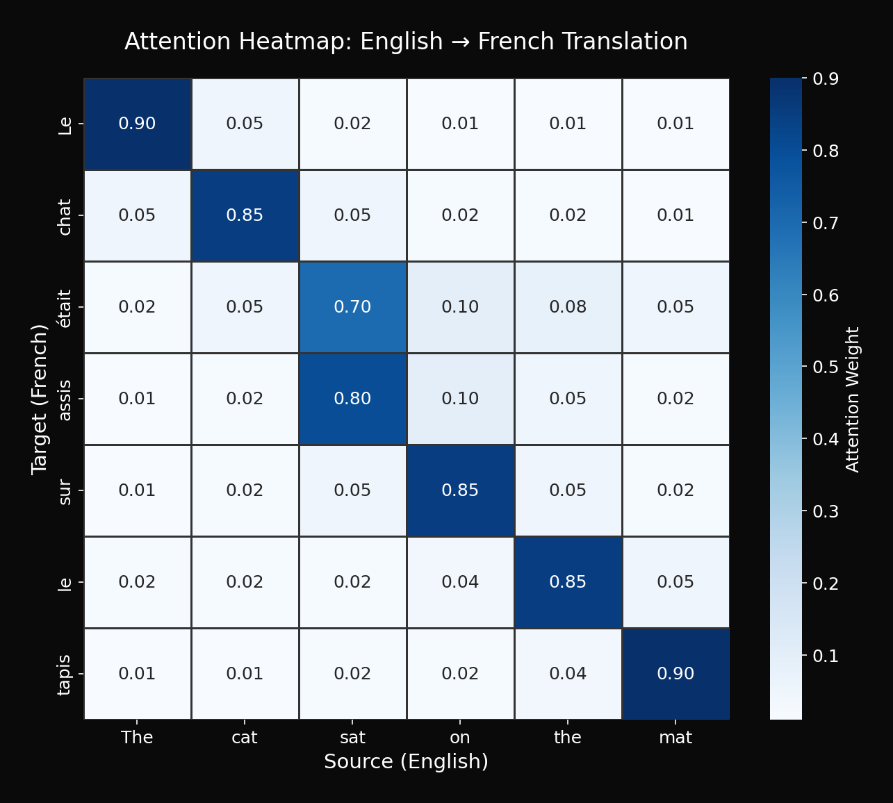
관찰:

"고양이가" → "cat"에 집중
"매트" → "mat"에 집중
"앉았다" → "sat"에 집중

이것이 Attention의 "설명 가능성(explainability)"입니다.

8. 고급 Attention 기법

8.1 Local Attention (Luong)

전체 인코더 출력이 아닌, 일부 창(window)만 참조:

$c_t = \sum_{i=p_t-D}^{p_t+D} \alpha_{ti} h_i^{enc}$

여기서 $p_t$ 는 예측된 alignment position, $D$ 는 window 크기

장점:

긴 시퀀스에서 메모리 효율적
계산량 감소

8.2 Multi-Head Attention (Preview)

여러 개의 attention을 병렬로 계산:

$\text{MultiHead}(Q, K, V) = \text{Concat}(\text{head}_1, ..., \text{head}_h) W^O$

이것이 나중에 Transformer의 핵심이 됩니다.

8.3 Self-Attention (Preview)

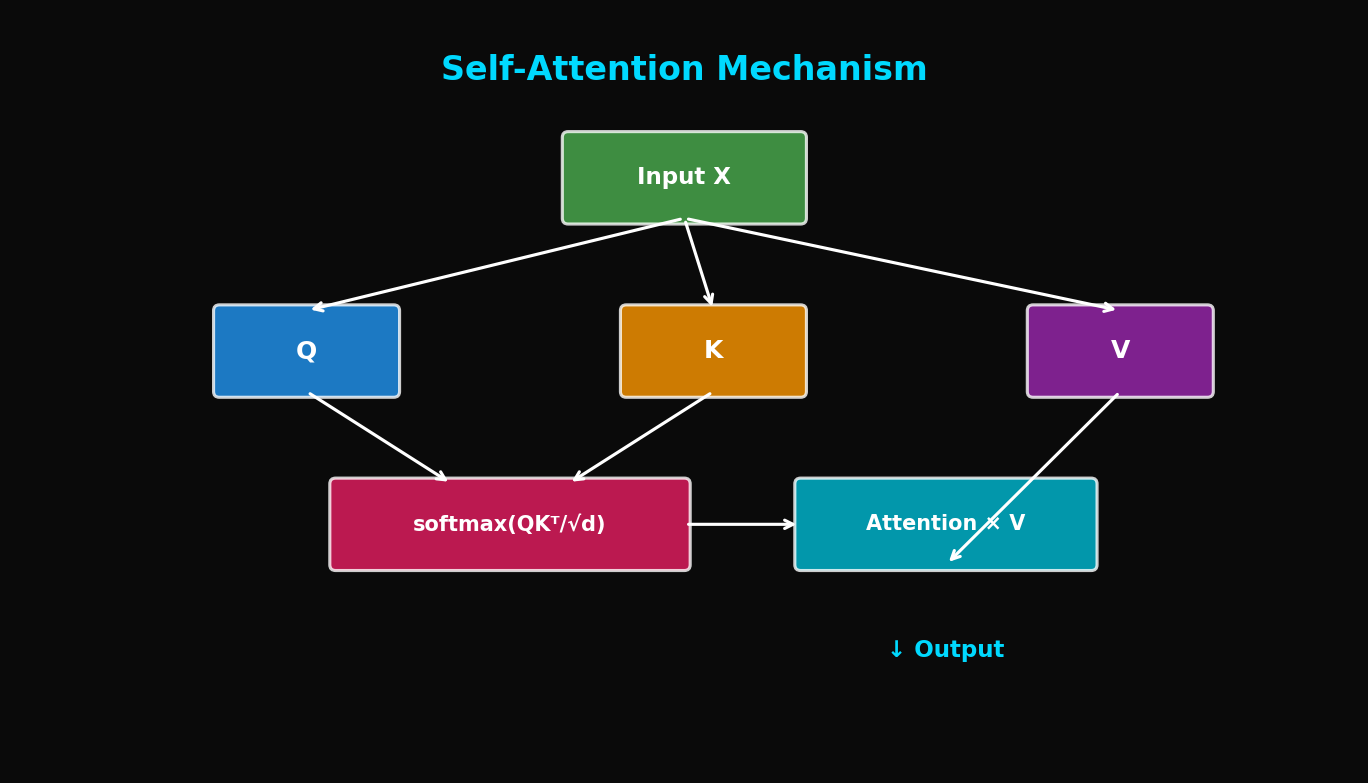
인코더/디코더 자기 자신에 대한 attention:

$\text{Attention}(Q, K, V) = \text{softmax}\left(\frac{QK^T}{\sqrt{d_k}}\right)V$

여기서 $Q = K = V$ 는 같은 시퀀스에서 유래

9. 실험 결과 분석

9.1 IWSLT 2016 English-German

Model	BLEU	Parameters
Seq2Seq (no attention)	22.3	15M
+ Bahdanau Attention	27.8	18M
+ Luong Dot	27.5	16M
+ Luong General	27.9	17M

9.2 문장 길이별 성능

문장 길이	No Attention	With Attention
1-10	25.3	26.1
11-20	22.1	26.8
21-30	18.7	26.4
31-40	14.2	25.9
41-50	10.5	24.8

핵심: Attention으로 긴 문장의 성능 저하가 크게 완화됨

9.3 학습 곡선

10. 실전 팁

10.1 어떤 Attention을 선택할까?

python

# 의사결정 트리
def choose_attention():
    if 속도가_중요:
        if encoder_dim == decoder_dim:
            return "Luong Dot"
        else:
            return "Luong General"
    elif 최고_성능_필요:
        return "Bahdanau"  # 또는 Luong Concat
    else:
        return "Luong General"  # 균형 잡힌 선택

10.2 Attention Dropout

Attention weight에 dropout을 적용하면 regularization 효과:

python

attn_weights = F.softmax(scores, dim=1)
attn_weights = F.dropout(attn_weights, p=0.1, training=self.training)
context = torch.bmm(attn_weights.unsqueeze(1), encoder_outputs).squeeze(1)

10.3 Padding Mask 적용

패딩 토큰에 attention이 가지 않도록:

python

def masked_attention(scores, mask):
    """
    scores: (batch, src_len)
    mask: (batch, src_len), True for padding positions
    """
    scores = scores.masked_fill(mask, float('-inf'))
    return F.softmax(scores, dim=1)

10.4 디버깅 체크리스트

□ Attention weights 합이 1인가?
□ Padding 위치의 attention weight가 0인가?
□ Attention heatmap이 합리적인 패턴을 보이는가?
□ 긴 문장에서 성능이 유지되는가?
□ Gradient가 안정적인가?

11. 결론

Attention은 NMT의 혁명이었습니다:

Context Vector 병목 해결: 동적 context 생성
긴 문장 처리 개선: 성능 저하 완화
해석 가능성: Attention heatmap으로 모델 이해

Bahdanau vs Luong:

이론적으로는 Bahdanau가 더 표현력 있음
실용적으로는 Luong Dot이 빠르고 충분히 좋음

다음 단계는 Self-Attention과 Transformer입니다. Attention을 극한까지 밀어붙인 결과가 오늘날의 GPT, BERT가 되었습니다.

References

Bahdanau, D., Cho, K., & Bengio, Y. (2015). Neural Machine Translation by Jointly Learning to Align and Translate. ICLR 2015
Luong, M. T., Pham, H., & Manning, C. D. (2015). Effective Approaches to Attention-based Neural Machine Translation. EMNLP 2015
Vaswani, A., et al. (2017). Attention Is All You Need. NeurIPS 2017
Xu, K., et al. (2015). Show, Attend and Tell: Neural Image Caption Generation with Visual Attention. ICML 2015

Tags: #Attention #Bahdanau #Luong #Seq2Seq #NMT #딥러닝 #자연어처리 #기계번역

이 글의 전체 코드는 첨부된 Jupyter Notebook에서 확인할 수 있습니다.