Complete Attention Mechanism Implementation: Bahdanau vs Luong, What's the Difference?

TL;DR: Attention allows the decoder to "reference" all encoder hidden states. Bahdanau uses additive scoring, Luong uses multiplicative. In practice, Luong is faster with similar performance.

1. Why Do We Need Attention?

1.1 The Seq2Seq Bottleneck: Context Vector

Let's revisit the basic Seq2Seq structure:

Encoder: [x₁, x₂, ..., xₙ] → h_n (context vector)
Decoder: h_n → [y₁, y₂, ..., yₘ]

Problem: No matter how long the sentence, it's compressed into a single fixed-size vector.

$c = h_n^{enc} \in \mathbb{R}^d$

This is like summarizing a 1000-page book into a 140-character tweet.

1.2 Performance Degradation on Long Sentences

Experimental results from Cho et al. (2014):

Sentence Length	BLEU Score
≤10	25.3
20	22.1
30	18.7
40	14.2
≥50	10.5

Performance drops dramatically as sentences get longer.

1.3 The Key Idea of Attention

"Focus on specific parts of the source when translating"

Think about how humans translate:

"I love machine learning" → "J'adore l'apprentissage automatique"
When translating "love" → "adore", focus on "love"
When translating "machine learning" → "apprentissage automatique", focus on those words

Attention implements this intuition mathematically.

2. Mathematical Foundations of Attention

2.1 Core Formula

The essence of Attention is a weighted average:

$c_t = \sum_{i=1}^{n} \alpha_{ti} \cdot h_i^{enc}$

Where:

$c_t$ : Context vector at time $t$ (dynamic!)
$\alpha_{ti}$ : Attention weight for encoder hidden state $i$ at time $t$
$h_i^{enc}$ : Encoder's $i$ -th hidden state

Key Point: The context vector is computed differently at each decoding step!

2.2 Computing Attention Weights

$\alpha_{ti} = \frac{\exp(e_{ti})}{\sum_{j=1}^{n} \exp(e_{tj})}$

Where $e_{ti}$ is the alignment score (or energy).

Through Softmax:

All weights sum to 1
Each weight is between 0 and 1
Can be interpreted as a "probability distribution"

2.3 Score Function: Bahdanau vs Luong

This is where the two approaches diverge. How to compute the score?

3. Bahdanau Attention (Additive)

3.1 Key Idea

Bahdanau et al. (2015) approach:

"Concatenate the decoder's previous hidden state with each encoder hidden state, then compute score through an MLP"

3.2 Mathematical Definition

$e_{ti} = v^T \tanh(W_s h_{t-1}^{dec} + W_h h_i^{enc})$

Where:

$h_{t-1}^{dec}$ : Decoder's previous hidden state
$h_i^{enc}$ : Encoder's $i$ -th hidden state
$W_s, W_h$ : Learnable weight matrices
$v$ : Learnable weight vector

3.3 Full Decoding Process

1. Run encoder: h₁, h₂, ..., hₙ (store all hidden states)
2. At each decoding step t:
a. Compute scores: e_ti = v^T tanh(W_s h_{t-1} + W_h h_i) for all i
b. Attention weights: α_ti = softmax(e_ti)
c. Context vector: c_t = Σ α_ti * h_i
d. Decoder input: [y_{t-1}; c_t] (concat)
e. Decoder output: h_t, y_t

3.4 PyTorch Implementation

python

class BahdanauAttention(nn.Module):
    def __init__(self, encoder_dim, decoder_dim, attention_dim):
        super().__init__()
        self.encoder_att = nn.Linear(encoder_dim, attention_dim, bias=False)
        self.decoder_att = nn.Linear(decoder_dim, attention_dim, bias=False)
        self.v = nn.Linear(attention_dim, 1, bias=False)

    def forward(self, encoder_outputs, decoder_hidden):
        """
        encoder_outputs: (batch, src_len, encoder_dim)
        decoder_hidden: (batch, decoder_dim)
        """
        # Expand decoder_hidden for src_len
        decoder_hidden = decoder_hidden.unsqueeze(1)  # (batch, 1, decoder_dim)

        # Compute scores
        encoder_proj = self.encoder_att(encoder_outputs)  # (batch, src_len, attention_dim)
        decoder_proj = self.decoder_att(decoder_hidden)   # (batch, 1, attention_dim)

        energy = torch.tanh(encoder_proj + decoder_proj)  # (batch, src_len, attention_dim)
        scores = self.v(energy).squeeze(-1)               # (batch, src_len)

        # Attention weights
        attn_weights = F.softmax(scores, dim=1)           # (batch, src_len)

        # Context vector
        context = torch.bmm(attn_weights.unsqueeze(1), encoder_outputs)
        context = context.squeeze(1)                       # (batch, encoder_dim)

        return context, attn_weights

3.5 Characteristics of Bahdanau

Advantages:

Theoretically more expressive (includes nonlinear transformation)
Validated in original paper

Disadvantages:

Higher computational cost (MLP operations)
More complex implementation

4. Luong Attention (Multiplicative)

4.1 Key Idea

Luong et al. (2015) approach:

"Compute score via dot product between the current decoder hidden state and encoder hidden states"

4.2 Three Score Functions

Luong proposed three score functions:

1. Dot Product:

$e_{ti} = h_t^{dec} \cdot h_i^{enc}$

2. General:

$e_{ti} = h_t^{dec} \cdot W_a \cdot h_i^{enc}$

3. Concat (similar to Bahdanau):

$e_{ti} = v^T \tanh(W_a [h_t^{dec}; h_i^{enc}])$

4.3 Full Decoding Process

1. Run encoder: h₁, h₂, ..., hₙ
2. At each decoding step t:
a. First run decoder: h_t = decoder(y_{t-1}, h_{t-1})
b. Compute scores: e_ti = h_t · W · h_i (or simple dot product)
c. Attention weights: α_ti = softmax(e_ti)
d. Context vector: c_t = Σ α_ti * h_i
e. Combine: h̃_t = tanh(W_c [c_t; h_t])
f. Output: y_t = softmax(W_o h̃_t)

Key Difference: Bahdanau uses $h_{t-1}$ , Luong uses $h_t$

4.4 PyTorch Implementation

python

class LuongAttention(nn.Module):
    def __init__(self, encoder_dim, decoder_dim, method='dot'):
        super().__init__()
        self.method = method

        if method == 'general':
            self.W = nn.Linear(encoder_dim, decoder_dim, bias=False)
        elif method == 'concat':
            self.W = nn.Linear(encoder_dim + decoder_dim, decoder_dim, bias=False)
            self.v = nn.Linear(decoder_dim, 1, bias=False)

    def forward(self, encoder_outputs, decoder_hidden):
        """
        encoder_outputs: (batch, src_len, encoder_dim)
        decoder_hidden: (batch, decoder_dim)
        """
        if self.method == 'dot':
            # (batch, src_len, encoder_dim) x (batch, encoder_dim, 1) -> (batch, src_len, 1)
            scores = torch.bmm(encoder_outputs, decoder_hidden.unsqueeze(2)).squeeze(2)

        elif self.method == 'general':
            # W*h_enc: (batch, src_len, decoder_dim)
            energy = self.W(encoder_outputs)
            scores = torch.bmm(energy, decoder_hidden.unsqueeze(2)).squeeze(2)

        elif self.method == 'concat':
            # Expand decoder hidden to match encoder outputs
            decoder_hidden_expanded = decoder_hidden.unsqueeze(1).expand(
                -1, encoder_outputs.size(1), -1
            )
            concat = torch.cat([encoder_outputs, decoder_hidden_expanded], dim=2)
            scores = self.v(torch.tanh(self.W(concat))).squeeze(2)

        # Attention weights
        attn_weights = F.softmax(scores, dim=1)

        # Context vector
        context = torch.bmm(attn_weights.unsqueeze(1), encoder_outputs).squeeze(1)

        return context, attn_weights

4.5 Characteristics of Luong

Advantages:

Faster computation (especially dot product)
Simpler implementation
Similar performance to Bahdanau in most cases

Disadvantages:

Requires encoder_dim == decoder_dim (for dot product)
Theoretically less expressive than Bahdanau

5. Bahdanau vs Luong: Detailed Comparison

5.1 Structural Differences

Property	Bahdanau	Luong
Hidden state	$h_{t-1}^{dec}$ (previous)	$h_t^{dec}$ (current)
Score function	Additive (MLP)	Multiplicative (dot/general)
Context combination	Concat to decoder input	Concat to decoder output
Computation order	Attention → Decoder	Decoder → Attention

5.2 Visual Comparison

Bahdanau:

Luong:

5.3 Performance Comparison (Original Papers)

WMT'14 English-German:

Model	BLEU
Base Seq2Seq	20.9
Bahdanau Attention	26.5
Luong (dot)	25.9
Luong (general)	26.2
Luong (concat)	26.4

Conclusion: Performance differences are minimal; Luong dot is most efficient for speed

5.4 Computational Complexity

Bahdanau:

$O(n \cdot d \cdot d_a) \quad \text{where } d_a \text{ is attention dimension}$

Luong Dot:

$O(n \cdot d)$

Luong is approximately $d_a$ times faster (typically $d_a \approx d$ )

6. Complete Attention Seq2Seq Implementation

6.1 Encoder (Bidirectional LSTM)

python

class AttentionEncoder(nn.Module):
    def __init__(self, vocab_size, embed_dim, hidden_dim, num_layers, dropout=0.1):
        super().__init__()
        self.embedding = nn.Embedding(vocab_size, embed_dim, padding_idx=0)
        self.lstm = nn.LSTM(
            embed_dim, hidden_dim, num_layers,
            batch_first=True, bidirectional=True, dropout=dropout
        )
        self.dropout = nn.Dropout(dropout)

        # Bidirectional -> Unidirectional projection
        self.fc_hidden = nn.Linear(hidden_dim * 2, hidden_dim)
        self.fc_cell = nn.Linear(hidden_dim * 2, hidden_dim)

    def forward(self, src, src_len):
        embedded = self.dropout(self.embedding(src))

        packed = nn.utils.rnn.pack_padded_sequence(
            embedded, src_len.cpu(), batch_first=True, enforce_sorted=False
        )
        outputs, (hidden, cell) = self.lstm(packed)
        outputs, _ = nn.utils.rnn.pad_packed_sequence(outputs, batch_first=True)

        # hidden: (num_layers*2, batch, hidden_dim)
        hidden = torch.cat([hidden[-2], hidden[-1]], dim=1)
        cell = torch.cat([cell[-2], cell[-1]], dim=1)

        hidden = torch.tanh(self.fc_hidden(hidden))
        cell = torch.tanh(self.fc_cell(cell))

        return outputs, hidden, cell

6.2 Decoder with Attention

python

class AttentionDecoder(nn.Module):
    def __init__(self, vocab_size, embed_dim, hidden_dim, encoder_dim,
                 attention_type='luong', attention_method='dot', dropout=0.1):
        super().__init__()
        self.vocab_size = vocab_size

        self.embedding = nn.Embedding(vocab_size, embed_dim, padding_idx=0)
        self.dropout = nn.Dropout(dropout)

        # Choose attention type
        if attention_type == 'bahdanau':
            self.attention = BahdanauAttention(encoder_dim, hidden_dim, hidden_dim)
            self.lstm = nn.LSTM(embed_dim + encoder_dim, hidden_dim, batch_first=True)
        else:  # luong
            self.attention = LuongAttention(encoder_dim, hidden_dim, attention_method)
            self.lstm = nn.LSTM(embed_dim, hidden_dim, batch_first=True)
            self.concat_layer = nn.Linear(hidden_dim + encoder_dim, hidden_dim)

        self.attention_type = attention_type
        self.fc_out = nn.Linear(hidden_dim, vocab_size)

    def forward(self, tgt, hidden, cell, encoder_outputs, mask=None):
        """
        tgt: (batch, 1)
        hidden, cell: (batch, hidden_dim)
        encoder_outputs: (batch, src_len, encoder_dim)
        """
        embedded = self.dropout(self.embedding(tgt))  # (batch, 1, embed_dim)

        if self.attention_type == 'bahdanau':
            # Bahdanau: Attention first, then Decoder
            context, attn_weights = self.attention(encoder_outputs, hidden)
            lstm_input = torch.cat([embedded, context.unsqueeze(1)], dim=2)
            output, (hidden, cell) = self.lstm(lstm_input, (hidden.unsqueeze(0), cell.unsqueeze(0)))
            hidden = hidden.squeeze(0)
            cell = cell.squeeze(0)

        else:  # luong
            # Luong: Decoder first, then Attention
            output, (hidden, cell) = self.lstm(embedded, (hidden.unsqueeze(0), cell.unsqueeze(0)))
            hidden = hidden.squeeze(0)
            cell = cell.squeeze(0)

            context, attn_weights = self.attention(encoder_outputs, hidden)
            concat_output = torch.cat([hidden, context], dim=1)
            hidden = torch.tanh(self.concat_layer(concat_output))

        prediction = self.fc_out(hidden)
        return prediction, hidden, cell, attn_weights

6.3 Full Model

python

class AttentionSeq2Seq(nn.Module):
    def __init__(self, encoder, decoder, device):
        super().__init__()
        self.encoder = encoder
        self.decoder = decoder
        self.device = device

    def forward(self, src, src_len, tgt, teacher_forcing_ratio=0.5):
        batch_size = src.size(0)
        tgt_len = tgt.size(1)
        vocab_size = self.decoder.vocab_size

        outputs = torch.zeros(batch_size, tgt_len, vocab_size).to(self.device)
        attentions = []

        # Encode
        encoder_outputs, hidden, cell = self.encoder(src, src_len)

        decoder_input = tgt[:, 0].unsqueeze(1)

        for t in range(1, tgt_len):
            output, hidden, cell, attn = self.decoder(
                decoder_input, hidden, cell, encoder_outputs
            )
            outputs[:, t] = output
            attentions.append(attn)

            teacher_force = torch.rand(1).item() < teacher_forcing_ratio
            top1 = output.argmax(1).unsqueeze(1)
            decoder_input = tgt[:, t].unsqueeze(1) if teacher_force else top1

        return outputs, torch.stack(attentions, dim=1)

7. Visualizing Attention

7.1 Attention Heatmap

Visualizing attention weights shows us "where the model is looking":

python

import matplotlib.pyplot as plt
import seaborn as sns

def visualize_attention(source, target, attention_weights):
    """
    source: Source token list
    target: Target token list
    attention_weights: (tgt_len, src_len) array
    """
    fig, ax = plt.subplots(figsize=(10, 8))

    sns.heatmap(
        attention_weights,
        xticklabels=source,
        yticklabels=target,
        cmap='Blues',
        ax=ax,
        square=True
    )

    ax.set_xlabel('Source (Input)')
    ax.set_ylabel('Target (Output)')
    ax.set_title('Attention Weights')

    # Rotate X-axis labels
    plt.xticks(rotation=45, ha='right')
    plt.tight_layout()

    return fig

7.2 Interpretation Example

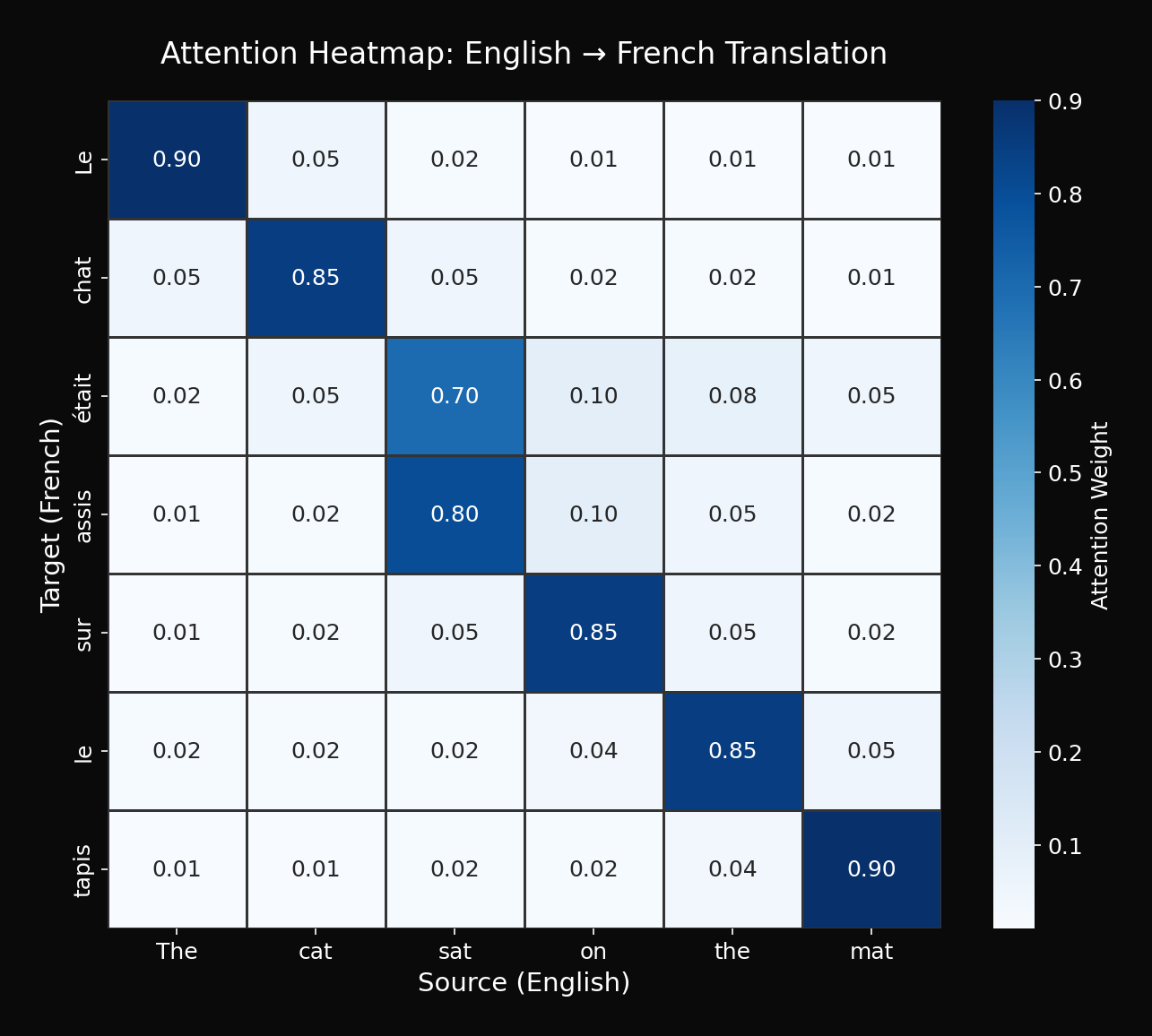
Attention Heatmap: English to French Translation

Observations:

"chat" → focuses on "cat"
"tapis" → focuses on "mat"
"assis" → focuses on "sat"

This is the "explainability" of Attention.

8. Advanced Attention Techniques

8.1 Local Attention (Luong)

Instead of all encoder outputs, reference only a window:

$c_t = \sum_{i=p_t-D}^{p_t+D} \alpha_{ti} h_i^{enc}$

Where $p_t$ is the predicted alignment position, $D$ is the window size

Advantages:

Memory efficient for long sequences
Reduced computation

8.2 Multi-Head Attention (Preview)

Compute multiple attention heads in parallel:

$\text{MultiHead}(Q, K, V) = \text{Concat}(\text{head}_1, ..., \text{head}_h) W^O$

This becomes the core of Transformer later.

8.3 Self-Attention (Preview)

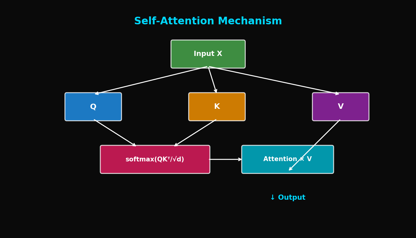
Attention on the same sequence (encoder/decoder to itself):

$\text{Attention}(Q, K, V) = \text{softmax}\left(\frac{QK^T}{\sqrt{d_k}}\right)V$

Where $Q = K = V$ come from the same sequence

9. Experimental Analysis

9.1 IWSLT 2016 English-German

Model	BLEU	Parameters
Seq2Seq (no attention)	22.3	15M
+ Bahdanau Attention	27.8	18M
+ Luong Dot	27.5	16M
+ Luong General	27.9	17M

9.2 Performance by Sentence Length

Sentence Length	No Attention	With Attention
1-10	25.3	26.1
11-20	22.1	26.8
21-30	18.7	26.4
31-40	14.2	25.9
41-50	10.5	24.8

Key Finding: Attention significantly mitigates performance degradation on long sentences

9.3 Training Curves

Training Progress: With vs Without Attention

10. Practical Tips

10.1 Which Attention Should You Choose?

python

# Decision tree
def choose_attention():
    if speed_matters:
        if encoder_dim == decoder_dim:
            return "Luong Dot"
        else:
            return "Luong General"
    elif need_best_performance:
        return "Bahdanau"  # or Luong Concat
    else:
        return "Luong General"  # Balanced choice

10.2 Attention Dropout

Applying dropout to attention weights provides regularization:

python

attn_weights = F.softmax(scores, dim=1)
attn_weights = F.dropout(attn_weights, p=0.1, training=self.training)
context = torch.bmm(attn_weights.unsqueeze(1), encoder_outputs).squeeze(1)

10.3 Applying Padding Mask

Prevent attention to padding tokens:

python

def masked_attention(scores, mask):
    """
    scores: (batch, src_len)
    mask: (batch, src_len), True for padding positions
    """
    scores = scores.masked_fill(mask, float('-inf'))
    return F.softmax(scores, dim=1)

10.4 Debugging Checklist

□ Do attention weights sum to 1?
□ Are attention weights 0 at padding positions?
□ Does the attention heatmap show reasonable patterns?
□ Is performance maintained on long sentences?
□ Are gradients stable?

11. Conclusion

Attention was a revolution in NMT:

Solved Context Vector Bottleneck: Dynamic context generation
Improved Long Sentence Processing: Mitigated performance degradation
Interpretability: Understanding models through attention heatmaps

Bahdanau vs Luong:

Theoretically, Bahdanau is more expressive
Practically, Luong Dot is fast and good enough

The next step is Self-Attention and Transformer. Pushing Attention to its limits led to today's GPT and BERT.

References

Bahdanau, D., Cho, K., & Bengio, Y. (2015). Neural Machine Translation by Jointly Learning to Align and Translate. ICLR 2015
Luong, M. T., Pham, H., & Manning, C. D. (2015). Effective Approaches to Attention-based Neural Machine Translation. EMNLP 2015
Vaswani, A., et al. (2017). Attention Is All You Need. NeurIPS 2017
Xu, K., et al. (2015). Show, Attend and Tell: Neural Image Caption Generation with Visual Attention. ICML 2015

Tags: #Attention #Bahdanau #Luong #Seq2Seq #NMT #Deep-Learning #NLP #Machine-Translation

The complete code for this article is available in the attached Jupyter Notebook.