DDIM으로 Diffusion 20배 빠르게: 품질 손실 없이 1000→50 스텝
DDPM pretrained 모델 그대로 쓰면서 샘플링만 20배 빠르게. 확률적→결정론적 변환의 수학적 원리와 eta 파라미터 튜닝 가이드.

DDIM: 빠른 Diffusion 샘플링, 1000 스텝을 50 스텝으로
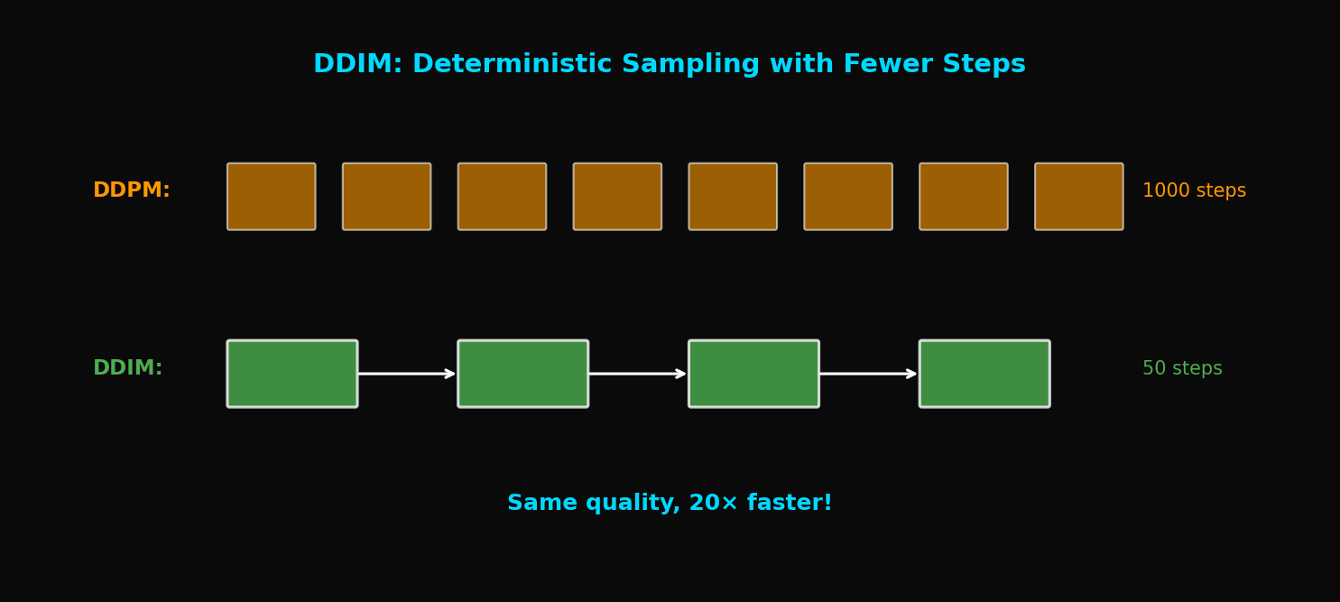
TL;DR: DDIM은 DDPM의 확률적 샘플링을 결정론적(deterministic)으로 바꿔 20배 빠른 샘플링을 가능하게 합니다. 동일한 pretrained 모델을 사용하면서도 품질 손실이 거의 없습니다.
1. DDPM의 속도 문제
1.1 왜 1000 스텝이 필요한가?
DDPM의 샘플링 과정:
문제: 각 스텝이 순차적으로 실행되어야 함
- GPU 병렬화 불가능
- 1000번의 forward pass 필요
- 이미지 1장에 ~20초
1.2 속도 vs 품질 Trade-off (DDPM)
DDPM에서 단순히 스텝 수를 줄이면?
| 스텝 수 | FID ↓ | 생성 시간 |
|---|---|---|
| 1000 | 3.17 | 20s |
| 500 | 4.82 | 10s |
| 100 | 15.3 | 2s |
| 50 | 35.7 | 1s |
품질이 급격히 저하됩니다.
1.3 DDIM의 핵심 통찰
Song et al.의 발견:
"DDPM의 학습된 모델은 더 일반적인 non-Markovian process를 정의한다. 이를 활용하면 더 적은 스텝으로 샘플링할 수 있다."
2. DDPM에서 DDIM으로
2.1 DDPM 복습
DDPM의 forward process:
Reverse process:
특징: 각 스텝에 노이즈를 추가하는 확률적(stochastic) 과정
2.2 일반화된 Forward Process
DDIM은 더 일반적인 forward process를 정의:
여기서:
핵심: 가 노이즈의 양을 조절
2.3 의 특별한 경우들
$\sigma_t = \sqrt{\frac{1-\bar{\alpha}_{t-1}}{1-\bar{\alpha}_t}} \sqrt{1-\frac{\bar{\alpha}_t}{\bar{\alpha}_{t-1}}}$ (DDPM):
원래 DDPM과 동일한 확률적 과정
$\sigma_t = 0$ (DDIM):
완전히 결정론적(deterministic)!
3. DDIM의 수학적 유도
3.1 예측된 계산
학습된 노이즈 예측 로부터:
이것은 현재 에서 추정한 원본 이미지입니다.
3.2 방향 벡터 계산
에서 를 향하는 방향:
3.3 DDIM Update Rule
다음 스텝으로 이동:
기하학적 해석:
3.4 Subsequence Sampling
DDIM의 진짜 힘: 임의의 subsequence 사용 가능
원래 [1, 2, 3, ..., 1000] 대신:
- [1, 21, 41, ..., 981] (50 steps)
- [1, 51, 101, ..., 951] (20 steps)
- [1, 101, 201, ..., 901] (10 steps)
def get_timestep_subsequence(total_steps, num_steps):
    """균등하게 분포된 timestep subsequence 생성"""
    c = total_steps // num_steps
    return list(range(0, total_steps, c))[:num_steps]

# 예: 1000 steps → 50 steps
subsequence = get_timestep_subsequence(1000, 50)
# [0, 20, 40, 60, ..., 980]
4. DDIM 구현
4.1 핵심 샘플링 코드
class DDIM:
    def __init__(self, model, T=1000, beta_start=1e-4, beta_end=0.02):
        self.model = model
        self.T = T

        # DDPM과 동일한 schedule
        betas = torch.linspace(beta_start, beta_end, T)
        alphas = 1 - betas
        self.alpha_bars = torch.cumprod(alphas, dim=0)

    @torch.no_grad()
    def sample(self, shape, device, num_steps=50, eta=0.0):
        """
        DDIM 샘플링

        Args:
            shape: 출력 shape (batch, channels, height, width)
            device: cuda/cpu
            num_steps: 샘플링 스텝 수
            eta: 노이즈 계수 (0=deterministic, 1=DDPM)
        """
        # Timestep subsequence 생성
        timesteps = self._get_timesteps(num_steps)

        # x_T ~ N(0, I)
        x = torch.randn(shape, device=device)

        for i in tqdm(range(len(timesteps) - 1, -1, -1)):
            t = timesteps[i]
            t_prev = timesteps[i - 1] if i > 0 else 0

            # 현재와 이전 alpha_bar
            alpha_bar = self.alpha_bars[t]
            alpha_bar_prev = self.alpha_bars[t_prev] if t_prev > 0 else torch.tensor(1.0)

            # 노이즈 예측
            t_batch = torch.full((shape[0],), t, device=device)
            epsilon_pred = self.model(x, t_batch)

            # x_0 예측
            x0_pred = (x - torch.sqrt(1 - alpha_bar) * epsilon_pred) / torch.sqrt(alpha_bar)
            x0_pred = torch.clamp(x0_pred, -1, 1)  # 범위 제한

            # 방향 (direction pointing to x_t)
            dir_xt = torch.sqrt(1 - alpha_bar_prev - eta**2 * self._get_variance(t, t_prev)) * epsilon_pred

            # Stochastic component (eta > 0일 때만)
            if eta > 0 and t > 0:
                noise = torch.randn_like(x)
                sigma = eta * torch.sqrt(self._get_variance(t, t_prev))
            else:
                noise = 0
                sigma = 0

            # DDIM update
            x = torch.sqrt(alpha_bar_prev) * x0_pred + dir_xt + sigma * noise

        return x

    def _get_timesteps(self, num_steps):
        """균등 간격 timestep 생성"""
        c = self.T // num_steps
        return list(range(0, self.T, c))

    def _get_variance(self, t, t_prev):
        """DDPM variance 계산"""
        alpha_bar = self.alpha_bars[t]
        alpha_bar_prev = self.alpha_bars[t_prev] if t_prev > 0 else torch.tensor(1.0)
        return (1 - alpha_bar_prev) / (1 - alpha_bar) * (1 - alpha_bar / alpha_bar_prev)
4.2 Eta () 파라미터
는 샘플링의 확률성을 조절:
| $\eta$ | 특성 | 용도 |
|---|---|---|
| 0 | 완전 결정론적 | Interpolation, Inversion |
| 1 | DDPM과 동일 | 다양성 필요시 |
| 0~1 | 중간 | Trade-off 조절 |
# 결정론적 샘플링 (재현 가능)
samples_deterministic = ddim.sample(shape, device, num_steps=50, eta=0.0)

# 확률적 샘플링 (더 다양)
samples_stochastic = ddim.sample(shape, device, num_steps=50, eta=1.0)
5. 실험 결과
5.1 스텝 수에 따른 품질 비교
CIFAR-10 FID:
| 스텝 수 | DDPM | DDIM ($\eta=0$) |
|---|---|---|
| 1000 | 3.17 | 4.16 |
| 100 | 15.3 | 4.67 |
| 50 | 35.7 | 4.89 |
| 20 | 78.2 | 6.84 |
| 10 | 143.5 | 13.36 |
DDIM이 50 스텝에서도 DDPM 1000 스텝과 비슷한 품질!
5.2 속도 향상
| 방법 | 스텝 | 시간 | FID |
|---|---|---|---|
| DDPM | 1000 | 20s | 3.17 |
| DDIM | 50 | 1s | 4.89 |
| DDIM | 20 | 0.4s | 6.84 |
20배 속도 향상 with minimal quality loss!
5.3 다양한 데이터셋 결과
| Dataset | Resolution | DDPM (1000) | DDIM (50) |
|---|---|---|---|
| CIFAR-10 | 32×32 | 3.17 | 4.89 |
| CelebA | 64×64 | 3.51 | 5.12 |
| LSUN Bedroom | 256×256 | 4.89 | 6.53 |
6. DDIM의 특별한 응용
6.1 결정론적 인코딩 (Inversion)
이면 과정이 가역적(invertible):
def ddim_inversion(ddim, x_0, num_steps=50):
    """이미지를 latent로 인코딩"""
    timesteps = ddim._get_timesteps(num_steps)

    x = x_0

    for i in range(len(timesteps) - 1):
        t = timesteps[i]
        t_next = timesteps[i + 1]

        alpha_bar = ddim.alpha_bars[t]
        alpha_bar_next = ddim.alpha_bars[t_next]

        # 노이즈 예측
        epsilon_pred = ddim.model(x, t)

        # x_0 예측
        x0_pred = (x - torch.sqrt(1 - alpha_bar) * epsilon_pred) / torch.sqrt(alpha_bar)

        # 다음 스텝으로 (역방향)
        x = torch.sqrt(alpha_bar_next) * x0_pred + torch.sqrt(1 - alpha_bar_next) * epsilon_pred

    return x  # x_T (latent)
6.2 이미지 보간 (Interpolation)
두 이미지 사이를 부드럽게 보간:
def interpolate_images(ddim, img1, img2, num_interp=5, num_steps=50):
    """두 이미지 사이 보간"""
    # 1. 두 이미지를 latent로 인코딩
    z1 = ddim_inversion(ddim, img1, num_steps)
    z2 = ddim_inversion(ddim, img2, num_steps)

    # 2. Latent space에서 선형 보간
    interpolations = []
    for alpha in torch.linspace(0, 1, num_interp):
        z_interp = (1 - alpha) * z1 + alpha * z2

        # 3. 보간된 latent를 이미지로 디코딩
        img_interp = ddim.sample_from_latent(z_interp, num_steps)
        interpolations.append(img_interp)

    return torch.stack(interpolations)
6.3 이미지 편집
def edit_image(ddim, image, edit_direction, strength=0.5, num_steps=50):
    """이미지 편집 (예: 나이 변화, 표정 변화)"""
    # 1. 이미지를 latent로 인코딩
    z = ddim_inversion(ddim, image, num_steps)

    # 2. Edit direction 적용
    z_edited = z + strength * edit_direction

    # 3. 편집된 latent를 이미지로 디코딩
    edited_image = ddim.sample_from_latent(z_edited, num_steps)

    return edited_image
7. 이론적 분석
7.1 왜 DDIM이 작동하는가?
핵심 통찰: DDPM의 학습 목표는 를 학습하는 것
이 목표는 샘플링 방식과 독립적입니다!
- DDPM: 확률적 샘플링
- DDIM: 결정론적 샘플링
- 둘 다 동일한 $\epsilon_\theta$ 사용
7.2 Non-Markovian Interpretation
DDIM의 reverse process:
에 대한 조건부 확률 → Non-Markovian
하지만 를 로 추정하므로 문제없음
7.3 ODE Formulation
연속 시간 한계에서 DDIM은 확률 ODE:
여기서
8. DDIM vs DDPM 비교
8.1 수학적 차이
| 속성 | DDPM | DDIM |
|---|---|---|
| 샘플링 | Stochastic | Deterministic ($\eta=0$) |
| Reverse process | Markovian | Non-Markovian |
| 연속 해석 | SDE | ODE |
| 가역성 | No | Yes |
8.2 실용적 차이
| 속성 | DDPM | DDIM |
|---|---|---|
| 최소 스텝 | ~1000 | ~20-50 |
| 다양성 | High | Controllable |
| 재현성 | No | Yes ($\eta=0$) |
| Inversion | Difficult | Easy |
8.3 언제 무엇을 쓸까?
DDPM 사용:
- 최고 품질이 필요할 때
- 다양성이 중요할 때
- 시간 제약이 없을 때
DDIM 사용:
- 빠른 샘플링이 필요할 때
- 이미지 편집/보간을 할 때
- 재현 가능한 결과가 필요할 때
9. 구현 팁
9.1 최적의 스텝 수 선택
def find_optimal_steps(ddim, val_images, step_options=[10, 20, 50, 100]):
    """품질과 속도의 최적 trade-off 찾기"""
    results = {}

    for num_steps in step_options:
        start = time.time()
        samples = ddim.sample(shape, device, num_steps=num_steps)
        elapsed = time.time() - start

        fid = calculate_fid(samples, val_images)
        results[num_steps] = {'fid': fid, 'time': elapsed}

    return results
경험적 권장:
- 빠른 프로토타이핑: 20 steps
- 일반적 사용: 50 steps
- 고품질 필요: 100 steps
9.2 선택
# 재현성이 중요: eta = 0
samples = ddim.sample(shape, device, eta=0.0)

# 다양성이 중요: eta > 0
samples = ddim.sample(shape, device, eta=0.5)

# DDPM과 동일한 다양성: eta = 1
samples = ddim.sample(shape, device, eta=1.0)
9.3 Classifier-Free Guidance와 결합
def ddim_sample_with_cfg(ddim, shape, device, num_steps, cfg_scale=7.5, condition=None):
    """Classifier-Free Guidance와 DDIM 결합"""
    x = torch.randn(shape, device=device)
    timesteps = ddim._get_timesteps(num_steps)

    for t in reversed(timesteps):
        # Unconditional과 conditional 예측
        eps_uncond = ddim.model(x, t, condition=None)
        eps_cond = ddim.model(x, t, condition=condition)

        # CFG 적용
        eps = eps_uncond + cfg_scale * (eps_cond - eps_uncond)

        # DDIM update (eps 사용)
        x = ddim_step(x, t, eps)

    return x
10. 결론
DDIM은 Diffusion 모델의 실용화에 결정적 기여를 했습니다:
- 20배 빠른 샘플링 (1000 → 50 steps)
- 품질 손실 최소화 (FID 3.17 → 4.89)
- 결정론적 인코딩 가능 (이미지 편집의 기반)
- 재현 가능한 결과
DDIM이 없었다면 Stable Diffusion도 없었을 것입니다. 다음 글에서는 Latent Diffusion을 다룹니다: 픽셀 공간이 아닌 latent 공간에서 diffusion을 수행하여 고해상도 이미지 생성을 가능하게 한 혁신.
References
- Song, J., Meng, C., & Ermon, S. (2021). Denoising Diffusion Implicit Models. ICLR 2021
- Ho, J., Jain, A., & Abbeel, P. (2020). Denoising Diffusion Probabilistic Models. NeurIPS 2020
- Song, Y., et al. (2021). Score-Based Generative Modeling through Stochastic Differential Equations. ICLR 2021
- Dhariwal, P., & Nichol, A. (2021). Diffusion Models Beat GANs on Image Synthesis. NeurIPS 2021
Tags: #DDIM #Diffusion #빠른샘플링 #딥러닝 #이미지생성 #결정론적샘플링 #ODE
이 글의 전체 코드는 첨부된 Jupyter Notebook에서 확인할 수 있습니다.
이메일로 받아보기
관련 포스트

SDFT: 자기 증류로 망각 없이 학습하기
복잡한 강화학습 없이, 모델이 스스로를 선생님 삼아 새로운 기술을 배우면서도 기존 능력을 유지하는 방법.

Qwen3-Max-Thinking 스냅샷 공개: 추론형 AI의 새로운 기준
최근 LLM 시장의 트렌드는 단순히 '더 많은 데이터'를 학습하는 것을 넘어, 모델이 '어떻게 생각하느냐'에 집중하고 있습니다. 알리바바 클라우드(Alibaba Cloud)가 자사의 가장 강력한 모델 Qwen3-Max-Thinking의 API 스냅샷(qwen3-max-2026-01-23)을 공개했습니다.

YOLO26: Upgrade or Hype? 완벽 가이드
2026년 1월 출시된 YOLO26의 핵심 기능, YOLO11과의 성능 비교, 그리고 실제 업그레이드 가치가 있는지 실습과 함께 분석합니다.