DDIM: Fast Diffusion Sampling - From 1000 Steps to 50 Steps

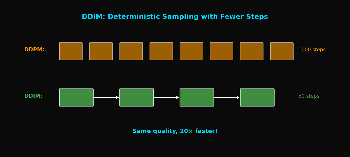
TL;DR: DDIM transforms DDPM's stochastic sampling into deterministic sampling, enabling 20x faster sampling. It uses the same pretrained model with nearly no quality loss.

1. DDPM's Speed Problem

1.1 Why Are 1000 Steps Necessary?

DDPM's sampling process:

Problem: Each step must be executed sequentially

• Cannot parallelize on GPU
• Requires 1000 forward passes
• ~20 seconds per image

1.2 Speed vs Quality Trade-off (DDPM)

What happens if we simply reduce steps in DDPM?

Quality degrades dramatically.

1.3 DDIM's Key Insight

Song et al.'s discovery:

"DDPM's trained model defines a more general non-Markovian process. By leveraging this, we can sample with fewer steps."

2. From DDPM to DDIM

2.1 DDPM Review

DDPM's forward process:

$$q(x_t | x_{t-1}) = \mathcal{N}(x_t; \sqrt{\alpha_t} x_{t-1}, (1-\alpha_t) I)$$

Reverse process:

$$p_\theta(x_{t-1} | x_t) = \mathcal{N}(x_{t-1}; \mu_\theta(x_t, t), \sigma_t^2 I)$$

Characteristic: A stochastic process that adds noise at each step

2.2 Generalized Forward Process

DDIM defines a more general forward process:

$$q_\sigma(x_{t-1} | x_t, x_0) = \mathcal{N}(x_{t-1}; \tilde{\mu}_t(x_t, x_0), \sigma_t^2 I)$$

Where:

$$\tilde{\mu}_t = \sqrt{\bar{\alpha}_{t-1}} x_0 + \sqrt{1 - \bar{\alpha}_{t-1} - \sigma_t^2} \cdot \frac{x_t - \sqrt{\bar{\alpha}_t} x_0}{\sqrt{1 - \bar{\alpha}_t}}$$

Key: $\sigma_t$ controls the amount of noise

2.3 Special Cases of $\sigma_t$

$\sigma_t = \sqrt{\frac{1-\bar{\alpha}_{t-1}}{1-\bar{\alpha}_t}} \sqrt{1-\frac{\bar{\alpha}_t}{\bar{\alpha}_{t-1}}}$ (DDPM):

Same stochastic process as original DDPM

$\sigma_t = 0$ (DDIM):

$$x_{t-1} = \sqrt{\bar{\alpha}_{t-1}} \underbrace{\left( \frac{x_t - \sqrt{1-\bar{\alpha}_t} \epsilon_\theta(x_t, t)}{\sqrt{\bar{\alpha}_t}} \right)}_{\text{predicted } x_0} + \sqrt{1 - \bar{\alpha}_{t-1}} \cdot \epsilon_\theta(x_t, t)$$

Completely deterministic!

3. Mathematical Derivation of DDIM

3.1 Computing Predicted $x_0$

From learned noise prediction $\epsilon_\theta(x_t, t)$:

$$\hat{x}_0 = \frac{x_t - \sqrt{1 - \bar{\alpha}_t} \epsilon_\theta(x_t, t)}{\sqrt{\bar{\alpha}_t}}$$

This is the estimated original image from current $x_t$.

3.2 Computing Direction Vector

Direction from $x_t$ toward $x_0$:

$$\text{direction} = \frac{x_t - \sqrt{\bar{\alpha}_t} \hat{x}_0}{\sqrt{1 - \bar{\alpha}_t}} = \epsilon_\theta(x_t, t)$$

3.3 DDIM Update Rule

Moving to next step:

$$x_{t-1} = \sqrt{\bar{\alpha}_{t-1}} \cdot \hat{x}_0 + \sqrt{1 - \bar{\alpha}_{t-1}} \cdot \epsilon_\theta(x_t, t)$$

Geometric Interpretation:

3.4 Subsequence Sampling

DDIM's true power: Can use arbitrary subsequences

Instead of [1, 2, 3, ..., 1000]:

• [1, 21, 41, ..., 981] (50 steps)
• [1, 51, 101, ..., 951] (20 steps)
• [1, 101, 201, ..., 901] (10 steps)

def get_timestep_subsequence(total_steps, num_steps):
    """Generate evenly distributed timestep subsequence"""
    c = total_steps // num_steps
    return list(range(0, total_steps, c))[:num_steps]

# Example: 1000 steps → 50 steps
subsequence = get_timestep_subsequence(1000, 50)
# [0, 20, 40, 60, ..., 980]

4. DDIM Implementation

4.1 Core Sampling Code

class DDIM:
    def __init__(self, model, T=1000, beta_start=1e-4, beta_end=0.02):
        self.model = model
        self.T = T

        # Same schedule as DDPM
        betas = torch.linspace(beta_start, beta_end, T)
        alphas = 1 - betas
        self.alpha_bars = torch.cumprod(alphas, dim=0)

    @torch.no_grad()
    def sample(self, shape, device, num_steps=50, eta=0.0):
        """
        DDIM Sampling

        Args:
            shape: Output shape (batch, channels, height, width)
            device: cuda/cpu
            num_steps: Number of sampling steps
            eta: Noise coefficient (0=deterministic, 1=DDPM)
        """
        # Generate timestep subsequence
        timesteps = self._get_timesteps(num_steps)

        # x_T ~ N(0, I)
        x = torch.randn(shape, device=device)

        for i in tqdm(range(len(timesteps) - 1, -1, -1)):
            t = timesteps[i]
            t_prev = timesteps[i - 1] if i > 0 else 0

            # Current and previous alpha_bar
            alpha_bar = self.alpha_bars[t]
            alpha_bar_prev = self.alpha_bars[t_prev] if t_prev > 0 else torch.tensor(1.0)

            # Predict noise
            t_batch = torch.full((shape[0],), t, device=device)
            epsilon_pred = self.model(x, t_batch)

            # Predict x_0
            x0_pred = (x - torch.sqrt(1 - alpha_bar) * epsilon_pred) / torch.sqrt(alpha_bar)
            x0_pred = torch.clamp(x0_pred, -1, 1)  # Clamp range

            # Direction (pointing to x_t)
            dir_xt = torch.sqrt(1 - alpha_bar_prev - eta**2 * self._get_variance(t, t_prev)) * epsilon_pred

            # Stochastic component (only when eta > 0)
            if eta > 0 and t > 0:
                noise = torch.randn_like(x)
                sigma = eta * torch.sqrt(self._get_variance(t, t_prev))
            else:
                noise = 0
                sigma = 0

            # DDIM update
            x = torch.sqrt(alpha_bar_prev) * x0_pred + dir_xt + sigma * noise

        return x

    def _get_timesteps(self, num_steps):
        """Generate evenly spaced timesteps"""
        c = self.T // num_steps
        return list(range(0, self.T, c))

    def _get_variance(self, t, t_prev):
        """Compute DDPM variance"""
        alpha_bar = self.alpha_bars[t]
        alpha_bar_prev = self.alpha_bars[t_prev] if t_prev > 0 else torch.tensor(1.0)
        return (1 - alpha_bar_prev) / (1 - alpha_bar) * (1 - alpha_bar / alpha_bar_prev)

4.2 Eta ($\eta$) Parameter

$\eta$ controls the stochasticity of sampling:

# Deterministic sampling (reproducible)
samples_deterministic = ddim.sample(shape, device, num_steps=50, eta=0.0)

# Stochastic sampling (more diverse)
samples_stochastic = ddim.sample(shape, device, num_steps=50, eta=1.0)

5. Experimental Results

5.1 Quality Comparison by Step Count

CIFAR-10 FID:

DDIM at 50 steps achieves similar quality to DDPM at 1000 steps!

5.2 Speed Improvement

20x speed improvement with minimal quality loss!

5.3 Results on Various Datasets

6. Special Applications of DDIM

6.1 Deterministic Encoding (Inversion)

When $\eta = 0$, the process is invertible:

$$x_0 \rightarrow x_T \rightarrow x_0' \approx x_0$$

def ddim_inversion(ddim, x_0, num_steps=50):
    """Encode image to latent"""
    timesteps = ddim._get_timesteps(num_steps)

    x = x_0

    for i in range(len(timesteps) - 1):
        t = timesteps[i]
        t_next = timesteps[i + 1]

        alpha_bar = ddim.alpha_bars[t]
        alpha_bar_next = ddim.alpha_bars[t_next]

        # Predict noise
        epsilon_pred = ddim.model(x, t)

        # Predict x_0
        x0_pred = (x - torch.sqrt(1 - alpha_bar) * epsilon_pred) / torch.sqrt(alpha_bar)

        # Move to next step (reverse direction)
        x = torch.sqrt(alpha_bar_next) * x0_pred + torch.sqrt(1 - alpha_bar_next) * epsilon_pred

    return x  # x_T (latent)

6.2 Image Interpolation

Smoothly interpolate between two images:

def interpolate_images(ddim, img1, img2, num_interp=5, num_steps=50):
    """Interpolate between two images"""
    # 1. Encode both images to latent
    z1 = ddim_inversion(ddim, img1, num_steps)
    z2 = ddim_inversion(ddim, img2, num_steps)

    # 2. Linear interpolation in latent space
    interpolations = []
    for alpha in torch.linspace(0, 1, num_interp):
        z_interp = (1 - alpha) * z1 + alpha * z2

        # 3. Decode interpolated latent to image
        img_interp = ddim.sample_from_latent(z_interp, num_steps)
        interpolations.append(img_interp)

    return torch.stack(interpolations)

6.3 Image Editing

def edit_image(ddim, image, edit_direction, strength=0.5, num_steps=50):
    """Edit image (e.g., age change, expression change)"""
    # 1. Encode image to latent
    z = ddim_inversion(ddim, image, num_steps)

    # 2. Apply edit direction
    z_edited = z + strength * edit_direction

    # 3. Decode edited latent to image
    edited_image = ddim.sample_from_latent(z_edited, num_steps)

    return edited_image

7. Theoretical Analysis

7.1 Why Does DDIM Work?

Key Insight: DDPM's training objective is to learn $\epsilon_\theta(x_t, t)$

$$\mathcal{L} = \mathbb{E}_{t, x_0, \epsilon} [ || \epsilon - \epsilon_\theta(x_t, t) ||^2 ]$$

This objective is independent of the sampling method!

• DDPM: Stochastic sampling
• DDIM: Deterministic sampling
• Both use the same $\epsilon_\theta$

7.2 Non-Markovian Interpretation

DDIM's reverse process:

$$q(x_{t-1} | x_t, x_0) \neq q(x_{t-1} | x_t)$$

Conditional on $x_0$ → Non-Markovian

But since we estimate $x_0$ with $\epsilon_\theta$, this is not a problem

7.3 ODE Formulation

In the continuous time limit, DDIM is a probability ODE:

$$dx = \left[ f(x, t) - \frac{1}{2} g(t)^2 \nabla_x \log p_t(x) \right] dt$$

Where $\nabla_x \log p_t(x) \approx -\epsilon_\theta(x, t) / \sqrt{1 - \bar{\alpha}_t}$

8. DDIM vs DDPM Comparison

8.1 Mathematical Differences

8.2 Practical Differences

8.3 When to Use Which?

Use DDPM:

• When highest quality is needed
• When diversity is important
• When there's no time constraint

Use DDIM:

• When fast sampling is needed
• When doing image editing/interpolation
• When reproducible results are needed

9. Implementation Tips

9.1 Choosing Optimal Step Count

def find_optimal_steps(ddim, val_images, step_options=[10, 20, 50, 100]):
    """Find optimal trade-off between quality and speed"""
    results = {}

    for num_steps in step_options:
        start = time.time()
        samples = ddim.sample(shape, device, num_steps=num_steps)
        elapsed = time.time() - start

        fid = calculate_fid(samples, val_images)
        results[num_steps] = {'fid': fid, 'time': elapsed}

    return results

Empirical Recommendations:

• Fast prototyping: 20 steps
• General use: 50 steps
• High quality needed: 100 steps

9.2 Choosing $\eta$

# Reproducibility important: eta = 0
samples = ddim.sample(shape, device, eta=0.0)

# Diversity important: eta > 0
samples = ddim.sample(shape, device, eta=0.5)

# Same diversity as DDPM: eta = 1
samples = ddim.sample(shape, device, eta=1.0)

9.3 Combining with Classifier-Free Guidance

def ddim_sample_with_cfg(ddim, shape, device, num_steps, cfg_scale=7.5, condition=None):
    """Combine Classifier-Free Guidance with DDIM"""
    x = torch.randn(shape, device=device)
    timesteps = ddim._get_timesteps(num_steps)

    for t in reversed(timesteps):
        # Unconditional and conditional predictions
        eps_uncond = ddim.model(x, t, condition=None)
        eps_cond = ddim.model(x, t, condition=condition)

        # Apply CFG
        eps = eps_uncond + cfg_scale * (eps_cond - eps_uncond)

        # DDIM update (using eps)
        x = ddim_step(x, t, eps)

    return x

10. Conclusion

DDIM made a decisive contribution to the practicalization of Diffusion models:

1. 20x faster sampling (1000 → 50 steps)
2. Minimal quality loss (FID 3.17 → 4.89)
3. Deterministic encoding possible (foundation for image editing)
4. Reproducible results

Without DDIM, there would be no Stable Diffusion. In the next article, we'll cover Latent Diffusion: the innovation that enabled high-resolution image generation by performing diffusion in latent space instead of pixel space.

References

1. Song, J., Meng, C., & Ermon, S. (2021). Denoising Diffusion Implicit Models. ICLR 2021
2. Ho, J., Jain, A., & Abbeel, P. (2020). Denoising Diffusion Probabilistic Models. NeurIPS 2020
3. Song, Y., et al. (2021). Score-Based Generative Modeling through Stochastic Differential Equations. ICLR 2021
4. Dhariwal, P., & Nichol, A. (2021). Diffusion Models Beat GANs on Image Synthesis. NeurIPS 2021

Tags: #DDIM #Diffusion #Fast-Sampling #Deep-Learning #Image-Generation #Deterministic-Sampling #ODE

The complete code for this article is available in the attached Jupyter Notebook.