DDPM: Diffusion 모델의 시작, 노이즈에서 이미지가 탄생하다

TL;DR: DDPM(Denoising Diffusion Probabilistic Model)은 이미지에 노이즈를 점진적으로 추가한 후, 이를 역으로 제거하여 이미지를 생성합니다. 수학적으로 엄밀하면서도 높은 품질의 이미지를 생성하는 혁명적 방법론입니다.

1. Diffusion Model이란?

1.1 생성 모델의 역사

딥러닝 기반 이미지 생성의 역사:

년도	모델	특징
2014	GAN	Adversarial training, mode collapse 문제
2014	VAE	Latent variable, blurry images
2016	PixelCNN	Autoregressive, 매우 느림
2019	Flow	Invertible networks, 메모리 intensive
2020	DDPM	Diffusion process, 고품질 + 안정적

1.2 핵심 아이디어

DDPM의 직관:

"이미지를 완전한 노이즈로 만드는 과정을 학습하고, 그 역과정을 수행하면 노이즈에서 이미지를 생성할 수 있다"

Forward Process (노이즈 추가):
x₀ (원본 이미지) → x₁ → x₂ → ... → x_T (순수 노이즈)

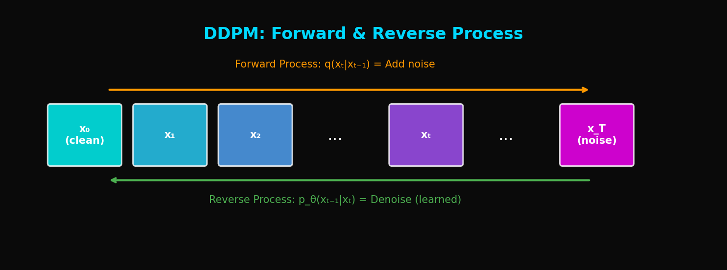
Reverse Process (노이즈 제거):
x_T (순수 노이즈) → x_{T-1} → ... → x₁ → x₀ (생성된 이미지)

1.3 왜 Diffusion인가?

물리학적 비유: 잉크가 물에 확산(diffusion)되는 과정을 생각하세요.

Forward: 잉크가 물에 퍼져 균일해짐 → 이미지가 노이즈로 변함
Reverse: 이 과정을 역으로 수행 → 노이즈에서 이미지가 응집

확률적 해석: 복잡한 데이터 분포 $p_{data}(x)$ 를 단순한 분포 $\mathcal{N}(0, I)$ 와 연결

2. 수학적 기초

2.1 Forward Process (Diffusion)

데이터 $x_0$ 에서 시작해 점진적으로 노이즈를 추가:

$q(x_t | x_{t-1}) = \mathcal{N}(x_t; \sqrt{1-\beta_t} x_{t-1}, \beta_t I)$

여기서:

$\beta_t$ : variance schedule (보통 $\beta_1 = 10^{-4}$ 에서 $\beta_T = 0.02$ 로 증가)
$T$ : 총 diffusion steps (보통 1000)

전체 forward process:

$q(x_{1:T} | x_0) = \prod_{t=1}^{T} q(x_t | x_{t-1})$

2.2 Key Insight: 어떤 시점으로든 직접 이동 가능

$\alpha_t = 1 - \beta_t$ , $\bar{\alpha}_t = \prod_{s=1}^{t} \alpha_s$ 로 정의하면:

$q(x_t | x_0) = \mathcal{N}(x_t; \sqrt{\bar{\alpha}_t} x_0, (1 - \bar{\alpha}_t) I)$

의미: $x_0$ 에서 $x_t$ 로 바로 갈 수 있음!

$x_t = \sqrt{\bar{\alpha}_t} x_0 + \sqrt{1 - \bar{\alpha}_t} \epsilon, \quad \epsilon \sim \mathcal{N}(0, I)$

2.3 Reverse Process (Denoising)

Forward process를 역으로:

$p_\theta(x_{t-1} | x_t) = \mathcal{N}(x_{t-1}; \mu_\theta(x_t, t), \Sigma_\theta(x_t, t))$

핵심 질문: $\mu_\theta$ 와 $\Sigma_\theta$ 를 어떻게 학습할까?

2.4 ELBO (Evidence Lower Bound)

log likelihood의 variational bound:

$\log p_\theta(x_0) \geq \mathbb{E}_{q} \left[ \log \frac{p_\theta(x_{0:T})}{q(x_{1:T}|x_0)} \right]$

이를 전개하면:

$\mathcal{L} = \underbrace{\mathbb{E}_q[\log p_\theta(x_0|x_1)]}_{\text{reconstruction}} - \underbrace{D_{KL}(q(x_T|x_0) || p(x_T))}_{\text{prior matching}} - \underbrace{\sum_{t=2}^{T} \mathbb{E}_q[D_{KL}(q(x_{t-1}|x_t,x_0) || p_\theta(x_{t-1}|x_t))]}_{\text{denoising matching}}$

2.5 Posterior 계산

Bayes' rule을 이용하면:

$q(x_{t-1} | x_t, x_0) = \mathcal{N}(x_{t-1}; \tilde{\mu}_t(x_t, x_0), \tilde{\beta}_t I)$

여기서:

$\tilde{\mu}_t(x_t, x_0) = \frac{\sqrt{\bar{\alpha}_{t-1}} \beta_t}{1 - \bar{\alpha}_t} x_0 + \frac{\sqrt{\alpha_t}(1 - \bar{\alpha}_{t-1})}{1 - \bar{\alpha}_t} x_t$

$\tilde{\beta}_t = \frac{1 - \bar{\alpha}_{t-1}}{1 - \bar{\alpha}_t} \beta_t$

3. 노이즈 예측으로의 재매개변수화

3.1 핵심 통찰

$x_t = \sqrt{\bar{\alpha}_t} x_0 + \sqrt{1 - \bar{\alpha}_t} \epsilon$ 이므로:

$x_0 = \frac{x_t - \sqrt{1 - \bar{\alpha}_t} \epsilon}{\sqrt{\bar{\alpha}_t}}$

따라서 $x_0$를 예측하는 대신 $\epsilon$을 예측하면:

$\tilde{\mu}_t = \frac{1}{\sqrt{\alpha_t}} \left( x_t - \frac{\beta_t}{\sqrt{1 - \bar{\alpha}_t}} \epsilon_\theta(x_t, t) \right)$

3.2 Simplified Loss

Ho et al.의 논문에서 제안한 간단한 loss:

$\mathcal{L}_{simple} = \mathbb{E}_{t, x_0, \epsilon} \left[ || \epsilon - \epsilon_\theta(x_t, t) ||^2 \right]$

해석: 네트워크가 추가된 노이즈를 예측하도록 학습

3.3 학습 알고리즘

python

def train_step(model, x_0):
    # 1. 랜덤 timestep 샘플링
    t = torch.randint(1, T+1, (batch_size,))

    # 2. 노이즈 샘플링
    epsilon = torch.randn_like(x_0)

    # 3. x_t 계산 (노이즈 추가)
    alpha_bar_t = get_alpha_bar(t)
    x_t = sqrt(alpha_bar_t) * x_0 + sqrt(1 - alpha_bar_t) * epsilon

    # 4. 노이즈 예측
    epsilon_pred = model(x_t, t)

    # 5. Loss 계산
    loss = F.mse_loss(epsilon_pred, epsilon)

    return loss

4. 샘플링 알고리즘

4.1 기본 샘플링

python

@torch.no_grad()
def sample(model, shape):
    # x_T ~ N(0, I)
    x = torch.randn(shape)

    for t in reversed(range(1, T+1)):
        # 노이즈 예측
        epsilon_pred = model(x, t)

        # μ_θ 계산
        alpha_t = get_alpha(t)
        alpha_bar_t = get_alpha_bar(t)
        beta_t = get_beta(t)

        mu = (1 / sqrt(alpha_t)) * (x - (beta_t / sqrt(1 - alpha_bar_t)) * epsilon_pred)

        # 노이즈 추가 (t > 1일 때만)
        if t > 1:
            sigma = sqrt(beta_t)
            x = mu + sigma * torch.randn_like(x)
        else:
            x = mu

    return x

4.2 Variance Schedule

Linear Schedule (원본 DDPM):

$\beta_t = \beta_1 + \frac{t-1}{T-1}(\beta_T - \beta_1)$

Cosine Schedule (Improved DDPM):

$\bar{\alpha}_t = \frac{f(t)}{f(0)}, \quad f(t) = \cos\left(\frac{t/T + s}{1 + s} \cdot \frac{\pi}{2}\right)^2$

python

def cosine_beta_schedule(timesteps, s=0.008):
    steps = timesteps + 1
    x = torch.linspace(0, timesteps, steps)
    alphas_cumprod = torch.cos(((x / timesteps) + s) / (1 + s) * torch.pi * 0.5) ** 2
    alphas_cumprod = alphas_cumprod / alphas_cumprod[0]
    betas = 1 - (alphas_cumprod[1:] / alphas_cumprod[:-1])
    return torch.clip(betas, 0.0001, 0.9999)

5. U-Net 아키텍처

5.1 전체 구조

DDPM에서 노이즈 예측 네트워크 $\epsilon_\theta$ 는 U-Net 구조:

5.2 Time Embedding

timestep $t$ 를 네트워크에 주입:

python

class SinusoidalPositionEmbeddings(nn.Module):
    def __init__(self, dim):
        super().__init__()
        self.dim = dim

    def forward(self, t):
        half_dim = self.dim // 2
        embeddings = math.log(10000) / (half_dim - 1)
        embeddings = torch.exp(torch.arange(half_dim) * -embeddings)
        embeddings = t[:, None] * embeddings[None, :]
        embeddings = torch.cat((embeddings.sin(), embeddings.cos()), dim=-1)
        return embeddings

5.3 ResNet Block with Time Conditioning

python

class ResBlock(nn.Module):
    def __init__(self, in_channels, out_channels, time_emb_dim):
        super().__init__()
        self.time_mlp = nn.Linear(time_emb_dim, out_channels)
        self.conv1 = nn.Conv2d(in_channels, out_channels, 3, padding=1)
        self.conv2 = nn.Conv2d(out_channels, out_channels, 3, padding=1)
        self.norm1 = nn.GroupNorm(8, out_channels)
        self.norm2 = nn.GroupNorm(8, out_channels)

        if in_channels != out_channels:
            self.shortcut = nn.Conv2d(in_channels, out_channels, 1)
        else:
            self.shortcut = nn.Identity()

    def forward(self, x, t_emb):
        h = self.conv1(x)
        h = self.norm1(h)
        h = h + self.time_mlp(t_emb)[:, :, None, None]  # Time conditioning
        h = F.silu(h)
        h = self.conv2(h)
        h = self.norm2(h)
        h = F.silu(h)
        return h + self.shortcut(x)

5.4 Self-Attention in U-Net

python

class SelfAttention(nn.Module):
    def __init__(self, channels, num_heads=4):
        super().__init__()
        self.mha = nn.MultiheadAttention(channels, num_heads, batch_first=True)
        self.ln = nn.LayerNorm(channels)

    def forward(self, x):
        b, c, h, w = x.shape
        x = x.view(b, c, h*w).transpose(1, 2)  # (B, H*W, C)
        x_ln = self.ln(x)
        attn_out, _ = self.mha(x_ln, x_ln, x_ln)
        x = x + attn_out
        return x.transpose(1, 2).view(b, c, h, w)

6. 완전한 구현

6.1 U-Net 전체 코드

python

class UNet(nn.Module):
    def __init__(self, in_channels=3, model_channels=64, out_channels=3,
                 channel_mult=(1, 2, 4, 8), attention_resolutions=(16, 8)):
        super().__init__()

        self.time_embed = nn.Sequential(
            SinusoidalPositionEmbeddings(model_channels),
            nn.Linear(model_channels, model_channels * 4),
            nn.SiLU(),
            nn.Linear(model_channels * 4, model_channels * 4),
        )

        # Encoder
        self.encoder = nn.ModuleList()
        ch = model_channels
        for level, mult in enumerate(channel_mult):
            for _ in range(2):
                self.encoder.append(ResBlock(ch, model_channels * mult, model_channels * 4))
                ch = model_channels * mult
            if level != len(channel_mult) - 1:
                self.encoder.append(Downsample(ch))

        # Bottleneck
        self.bottleneck = nn.Sequential(
            ResBlock(ch, ch, model_channels * 4),
            SelfAttention(ch),
            ResBlock(ch, ch, model_channels * 4),
        )

        # Decoder
        self.decoder = nn.ModuleList()
        for level, mult in reversed(list(enumerate(channel_mult))):
            for i in range(3):
                skip_ch = ch if i == 0 else model_channels * mult
                self.decoder.append(ResBlock(ch + skip_ch, model_channels * mult, model_channels * 4))
                ch = model_channels * mult
            if level != 0:
                self.decoder.append(Upsample(ch))

        self.out = nn.Sequential(
            nn.GroupNorm(8, ch),
            nn.SiLU(),
            nn.Conv2d(ch, out_channels, 3, padding=1),
        )

    def forward(self, x, t):
        t_emb = self.time_embed(t)

        # Encoder with skip connections
        skips = []
        for module in self.encoder:
            if isinstance(module, ResBlock):
                x = module(x, t_emb)
                skips.append(x)
            else:  # Downsample
                x = module(x)

        # Bottleneck
        x = self.bottleneck[0](x, t_emb)
        x = self.bottleneck[1](x)
        x = self.bottleneck[2](x, t_emb)

        # Decoder with skip connections
        for module in self.decoder:
            if isinstance(module, ResBlock):
                x = torch.cat([x, skips.pop()], dim=1)
                x = module(x, t_emb)
            else:  # Upsample
                x = module(x)

        return self.out(x)

6.2 DDPM 클래스

python

class DDPM:
    def __init__(self, model, T=1000, beta_start=1e-4, beta_end=0.02):
        self.model = model
        self.T = T

        # Variance schedule
        self.betas = torch.linspace(beta_start, beta_end, T)
        self.alphas = 1 - self.betas
        self.alpha_bars = torch.cumprod(self.alphas, dim=0)

    def get_loss(self, x_0):
        batch_size = x_0.shape[0]
        t = torch.randint(1, self.T + 1, (batch_size,))

        epsilon = torch.randn_like(x_0)
        alpha_bar = self.alpha_bars[t - 1].view(-1, 1, 1, 1)

        x_t = torch.sqrt(alpha_bar) * x_0 + torch.sqrt(1 - alpha_bar) * epsilon
        epsilon_pred = self.model(x_t, t)

        return F.mse_loss(epsilon_pred, epsilon)

    @torch.no_grad()
    def sample(self, shape, device):
        x = torch.randn(shape, device=device)

        for t in tqdm(reversed(range(1, self.T + 1))):
            t_batch = torch.full((shape[0],), t, device=device)
            epsilon_pred = self.model(x, t_batch)

            alpha = self.alphas[t - 1]
            alpha_bar = self.alpha_bars[t - 1]
            beta = self.betas[t - 1]

            mu = (1 / torch.sqrt(alpha)) * (x - (beta / torch.sqrt(1 - alpha_bar)) * epsilon_pred)

            if t > 1:
                sigma = torch.sqrt(beta)
                x = mu + sigma * torch.randn_like(x)
            else:
                x = mu

        return x

7. 실험 결과

7.1 CIFAR-10 벤치마크

Model	FID ↓	IS ↑
GAN (BigGAN)	14.73	9.22
VAE	78.51	-
PixelCNN	65.93	4.60
DDPM	3.17	9.46

DDPM이 압도적으로 좋은 FID를 달성!

7.2 샘플 품질

DDPM이 생성한 이미지의 특징:

다양성: mode collapse 없이 다양한 샘플
디테일: 고해상도에서도 선명한 디테일
안정성: 학습이 안정적

7.3 단점: 샘플링 속도

Model	샘플링 시간 (1 이미지)
GAN	~0.01초
VAE	~0.01초
DDPM (T=1000)	~20초

1000 스텝을 거쳐야 하므로 매우 느림 → DDIM에서 해결

8. DDPM의 의의와 한계

8.1 혁신적 기여

이론적 기반: 확률론적으로 엄밀한 framework
학습 안정성: GAN처럼 adversarial training 불필요
샘플 품질: SOTA FID 달성
다양성: Mode collapse 없음

8.2 한계점

느린 샘플링: 1000 steps 필요
고해상도 어려움: 픽셀 공간에서 직접 작동
조건부 생성 어려움: 기본 모델은 unconditional

8.3 후속 연구 방향

문제	해결책	논문
느린 샘플링	DDIM	Song et al. 2021
고해상도	Latent Diffusion	Rombach et al. 2022
조건부 생성	Classifier Guidance	Dhariwal et al. 2021
더 빠른 샘플링	Consistency Models	Song et al. 2023

9. 코드 실행 예제

9.1 학습

python

# 설정
device = torch.device('cuda' if torch.cuda.is_available() else 'cpu')
model = UNet().to(device)
ddpm = DDPM(model)
optimizer = torch.optim.Adam(model.parameters(), lr=2e-4)

# 학습 루프
for epoch in range(100):
    for batch in dataloader:
        x_0 = batch[0].to(device)
        loss = ddpm.get_loss(x_0)

        optimizer.zero_grad()
        loss.backward()
        optimizer.step()

    print(f"Epoch {epoch}: Loss = {loss.item():.4f}")

9.2 샘플링

python

# 샘플 생성
samples = ddpm.sample(shape=(16, 3, 32, 32), device=device)

# 이미지 저장
save_image(samples, 'samples.png', nrow=4, normalize=True)

10. 결론

DDPM은 생성 모델의 패러다임을 바꿨습니다:

노이즈 추가/제거라는 간단한 아이디어
확률론적으로 엄밀한 framework
GAN을 뛰어넘는 이미지 품질
안정적인 학습

하지만 1000 스텝 샘플링이라는 치명적 단점이 있습니다. 다음 글에서는 이를 50 스텝으로 줄이는 DDIM을 다룹니다.

References

Ho, J., Jain, A., & Abbeel, P. (2020). Denoising Diffusion Probabilistic Models. NeurIPS 2020
Sohl-Dickstein, J., et al. (2015). Deep Unsupervised Learning using Nonequilibrium Thermodynamics. ICML 2015
Song, Y., & Ermon, S. (2019). Generative Modeling by Estimating Gradients of the Data Distribution. NeurIPS 2019
Nichol, A., & Dhariwal, P. (2021). Improved Denoising Diffusion Probabilistic Models. ICML 2021

Tags: #DDPM #Diffusion #생성모델 #딥러닝 #이미지생성 #U-Net #노이즈제거

이 글의 전체 코드는 첨부된 Jupyter Notebook에서 확인할 수 있습니다.