DDPM: The Beginning of Diffusion Models - Images Born from Noise

TL;DR: DDPM (Denoising Diffusion Probabilistic Model) progressively adds noise to images, then learns to reverse this process to generate images from noise. It's a revolutionary methodology that is mathematically rigorous while producing high-quality images.

1. What is a Diffusion Model?

1.1 History of Generative Models

The history of deep learning-based image generation:

Year	Model	Characteristics
2014	GAN	Adversarial training, mode collapse issues
2014	VAE	Latent variables, blurry images
2016	PixelCNN	Autoregressive, very slow
2019	Flow	Invertible networks, memory intensive
2020	DDPM	Diffusion process, high quality + stable

1.2 Core Idea

The intuition behind DDPM:

"If we learn the process of turning an image into pure noise, we can reverse that process to generate images from noise"

Forward Process (Adding Noise):
x₀ (original image) → x₁ → x₂ → ... → x_T (pure noise)

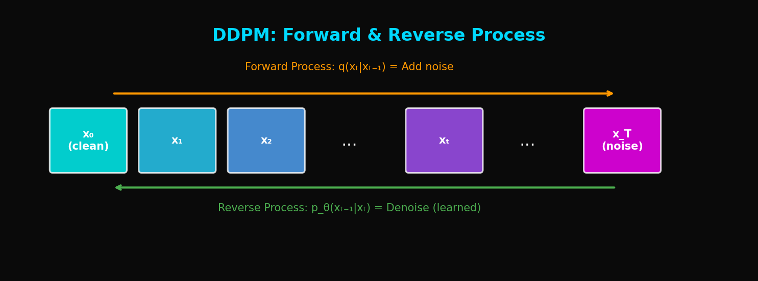
Reverse Process (Removing Noise):
x_T (pure noise) → x_{T-1} → ... → x₁ → x₀ (generated image)

1.3 Why "Diffusion"?

Physical Analogy: Think of ink diffusing in water.

Forward: Ink spreads in water becoming uniform → Image becomes noise
Reverse: Reversing this process → Image coalesces from noise

Probabilistic Interpretation: Connecting complex data distribution $p_{data}(x)$ to simple distribution $\mathcal{N}(0, I)$

2. Mathematical Foundations

2.1 Forward Process (Diffusion)

Starting from data $x_0$ , progressively add noise:

$q(x_t | x_{t-1}) = \mathcal{N}(x_t; \sqrt{1-\beta_t} x_{t-1}, \beta_t I)$

Where:

$\beta_t$ : variance schedule (typically $\beta_1 = 10^{-4}$ to $\beta_T = 0.02$ )
$T$ : total diffusion steps (typically 1000)

Full forward process:

$q(x_{1:T} | x_0) = \prod_{t=1}^{T} q(x_t | x_{t-1})$

2.2 Key Insight: Direct Jump to Any Timestep

Defining $\alpha_t = 1 - \beta_t$ , $\bar{\alpha}_t = \prod_{s=1}^{t} \alpha_s$ :

$q(x_t | x_0) = \mathcal{N}(x_t; \sqrt{\bar{\alpha}_t} x_0, (1 - \bar{\alpha}_t) I)$

Meaning: We can go directly from $x_0$ to $x_t$ !

$x_t = \sqrt{\bar{\alpha}_t} x_0 + \sqrt{1 - \bar{\alpha}_t} \epsilon, \quad \epsilon \sim \mathcal{N}(0, I)$

2.3 Reverse Process (Denoising)

Reversing the forward process:

$p_\theta(x_{t-1} | x_t) = \mathcal{N}(x_{t-1}; \mu_\theta(x_t, t), \Sigma_\theta(x_t, t))$

Key Question: How do we learn $\mu_\theta$ and $\Sigma_\theta$ ?

2.4 ELBO (Evidence Lower Bound)

Variational bound on log likelihood:

$\log p_\theta(x_0) \geq \mathbb{E}_{q} \left[ \log \frac{p_\theta(x_{0:T})}{q(x_{1:T}|x_0)} \right]$

Expanding this:

$\mathcal{L} = \underbrace{\mathbb{E}_q[\log p_\theta(x_0|x_1)]}_{\text{reconstruction}} - \underbrace{D_{KL}(q(x_T|x_0) || p(x_T))}_{\text{prior matching}} - \underbrace{\sum_{t=2}^{T} \mathbb{E}_q[D_{KL}(q(x_{t-1}|x_t,x_0) || p_\theta(x_{t-1}|x_t))]}_{\text{denoising matching}}$

2.5 Posterior Computation

Using Bayes' rule:

$q(x_{t-1} | x_t, x_0) = \mathcal{N}(x_{t-1}; \tilde{\mu}_t(x_t, x_0), \tilde{\beta}_t I)$

Where:

$\tilde{\mu}_t(x_t, x_0) = \frac{\sqrt{\bar{\alpha}_{t-1}} \beta_t}{1 - \bar{\alpha}_t} x_0 + \frac{\sqrt{\alpha_t}(1 - \bar{\alpha}_{t-1})}{1 - \bar{\alpha}_t} x_t$

$\tilde{\beta}_t = \frac{1 - \bar{\alpha}_{t-1}}{1 - \bar{\alpha}_t} \beta_t$

3. Reparameterization to Noise Prediction

3.1 Key Insight

Since $x_t = \sqrt{\bar{\alpha}_t} x_0 + \sqrt{1 - \bar{\alpha}_t} \epsilon$ :

$x_0 = \frac{x_t - \sqrt{1 - \bar{\alpha}_t} \epsilon}{\sqrt{\bar{\alpha}_t}}$

Therefore, instead of predicting $x_0$, predict $\epsilon$:

$\tilde{\mu}_t = \frac{1}{\sqrt{\alpha_t}} \left( x_t - \frac{\beta_t}{\sqrt{1 - \bar{\alpha}_t}} \epsilon_\theta(x_t, t) \right)$

3.2 Simplified Loss

The simple loss proposed by Ho et al.:

$\mathcal{L}_{simple} = \mathbb{E}_{t, x_0, \epsilon} \left[ || \epsilon - \epsilon_\theta(x_t, t) ||^2 \right]$

Interpretation: Train the network to predict the added noise

3.3 Training Algorithm

python

def train_step(model, x_0):
    # 1. Sample random timestep
    t = torch.randint(1, T+1, (batch_size,))

    # 2. Sample noise
    epsilon = torch.randn_like(x_0)

    # 3. Compute x_t (add noise)
    alpha_bar_t = get_alpha_bar(t)
    x_t = sqrt(alpha_bar_t) * x_0 + sqrt(1 - alpha_bar_t) * epsilon

    # 4. Predict noise
    epsilon_pred = model(x_t, t)

    # 5. Compute loss
    loss = F.mse_loss(epsilon_pred, epsilon)

    return loss

4. Sampling Algorithm

4.1 Basic Sampling

python

@torch.no_grad()
def sample(model, shape):
    # x_T ~ N(0, I)
    x = torch.randn(shape)

    for t in reversed(range(1, T+1)):
        # Predict noise
        epsilon_pred = model(x, t)

        # Compute μ_θ
        alpha_t = get_alpha(t)
        alpha_bar_t = get_alpha_bar(t)
        beta_t = get_beta(t)

        mu = (1 / sqrt(alpha_t)) * (x - (beta_t / sqrt(1 - alpha_bar_t)) * epsilon_pred)

        # Add noise (only when t > 1)
        if t > 1:
            sigma = sqrt(beta_t)
            x = mu + sigma * torch.randn_like(x)
        else:
            x = mu

    return x

4.2 Variance Schedule

Linear Schedule (Original DDPM):

$\beta_t = \beta_1 + \frac{t-1}{T-1}(\beta_T - \beta_1)$

Cosine Schedule (Improved DDPM):

$\bar{\alpha}_t = \frac{f(t)}{f(0)}, \quad f(t) = \cos\left(\frac{t/T + s}{1 + s} \cdot \frac{\pi}{2}\right)^2$

python

def cosine_beta_schedule(timesteps, s=0.008):
    steps = timesteps + 1
    x = torch.linspace(0, timesteps, steps)
    alphas_cumprod = torch.cos(((x / timesteps) + s) / (1 + s) * torch.pi * 0.5) ** 2
    alphas_cumprod = alphas_cumprod / alphas_cumprod[0]
    betas = 1 - (alphas_cumprod[1:] / alphas_cumprod[:-1])
    return torch.clip(betas, 0.0001, 0.9999)

5. U-Net Architecture

5.1 Overall Structure

The noise prediction network $\epsilon_\theta$ in DDPM uses a U-Net structure:

5.2 Time Embedding

Injecting timestep $t$ into the network:

python

class SinusoidalPositionEmbeddings(nn.Module):
    def __init__(self, dim):
        super().__init__()
        self.dim = dim

    def forward(self, t):
        half_dim = self.dim // 2
        embeddings = math.log(10000) / (half_dim - 1)
        embeddings = torch.exp(torch.arange(half_dim) * -embeddings)
        embeddings = t[:, None] * embeddings[None, :]
        embeddings = torch.cat((embeddings.sin(), embeddings.cos()), dim=-1)
        return embeddings

5.3 ResNet Block with Time Conditioning

python

class ResBlock(nn.Module):
    def __init__(self, in_channels, out_channels, time_emb_dim):
        super().__init__()
        self.time_mlp = nn.Linear(time_emb_dim, out_channels)
        self.conv1 = nn.Conv2d(in_channels, out_channels, 3, padding=1)
        self.conv2 = nn.Conv2d(out_channels, out_channels, 3, padding=1)
        self.norm1 = nn.GroupNorm(8, out_channels)
        self.norm2 = nn.GroupNorm(8, out_channels)

        if in_channels != out_channels:
            self.shortcut = nn.Conv2d(in_channels, out_channels, 1)
        else:
            self.shortcut = nn.Identity()

    def forward(self, x, t_emb):
        h = self.conv1(x)
        h = self.norm1(h)
        h = h + self.time_mlp(t_emb)[:, :, None, None]  # Time conditioning
        h = F.silu(h)
        h = self.conv2(h)
        h = self.norm2(h)
        h = F.silu(h)
        return h + self.shortcut(x)

5.4 Self-Attention in U-Net

python

class SelfAttention(nn.Module):
    def __init__(self, channels, num_heads=4):
        super().__init__()
        self.mha = nn.MultiheadAttention(channels, num_heads, batch_first=True)
        self.ln = nn.LayerNorm(channels)

    def forward(self, x):
        b, c, h, w = x.shape
        x = x.view(b, c, h*w).transpose(1, 2)  # (B, H*W, C)
        x_ln = self.ln(x)
        attn_out, _ = self.mha(x_ln, x_ln, x_ln)
        x = x + attn_out
        return x.transpose(1, 2).view(b, c, h, w)

6. Complete Implementation

6.1 Full U-Net Code

python

class UNet(nn.Module):
    def __init__(self, in_channels=3, model_channels=64, out_channels=3,
                 channel_mult=(1, 2, 4, 8), attention_resolutions=(16, 8)):
        super().__init__()

        self.time_embed = nn.Sequential(
            SinusoidalPositionEmbeddings(model_channels),
            nn.Linear(model_channels, model_channels * 4),
            nn.SiLU(),
            nn.Linear(model_channels * 4, model_channels * 4),
        )

        # Encoder
        self.encoder = nn.ModuleList()
        ch = model_channels
        for level, mult in enumerate(channel_mult):
            for _ in range(2):
                self.encoder.append(ResBlock(ch, model_channels * mult, model_channels * 4))
                ch = model_channels * mult
            if level != len(channel_mult) - 1:
                self.encoder.append(Downsample(ch))

        # Bottleneck
        self.bottleneck = nn.Sequential(
            ResBlock(ch, ch, model_channels * 4),
            SelfAttention(ch),
            ResBlock(ch, ch, model_channels * 4),
        )

        # Decoder
        self.decoder = nn.ModuleList()
        for level, mult in reversed(list(enumerate(channel_mult))):
            for i in range(3):
                skip_ch = ch if i == 0 else model_channels * mult
                self.decoder.append(ResBlock(ch + skip_ch, model_channels * mult, model_channels * 4))
                ch = model_channels * mult
            if level != 0:
                self.decoder.append(Upsample(ch))

        self.out = nn.Sequential(
            nn.GroupNorm(8, ch),
            nn.SiLU(),
            nn.Conv2d(ch, out_channels, 3, padding=1),
        )

    def forward(self, x, t):
        t_emb = self.time_embed(t)

        # Encoder with skip connections
        skips = []
        for module in self.encoder:
            if isinstance(module, ResBlock):
                x = module(x, t_emb)
                skips.append(x)
            else:  # Downsample
                x = module(x)

        # Bottleneck
        x = self.bottleneck[0](x, t_emb)
        x = self.bottleneck[1](x)
        x = self.bottleneck[2](x, t_emb)

        # Decoder with skip connections
        for module in self.decoder:
            if isinstance(module, ResBlock):
                x = torch.cat([x, skips.pop()], dim=1)
                x = module(x, t_emb)
            else:  # Upsample
                x = module(x)

        return self.out(x)

6.2 DDPM Class

python

class DDPM:
    def __init__(self, model, T=1000, beta_start=1e-4, beta_end=0.02):
        self.model = model
        self.T = T

        # Variance schedule
        self.betas = torch.linspace(beta_start, beta_end, T)
        self.alphas = 1 - self.betas
        self.alpha_bars = torch.cumprod(self.alphas, dim=0)

    def get_loss(self, x_0):
        batch_size = x_0.shape[0]
        t = torch.randint(1, self.T + 1, (batch_size,))

        epsilon = torch.randn_like(x_0)
        alpha_bar = self.alpha_bars[t - 1].view(-1, 1, 1, 1)

        x_t = torch.sqrt(alpha_bar) * x_0 + torch.sqrt(1 - alpha_bar) * epsilon
        epsilon_pred = self.model(x_t, t)

        return F.mse_loss(epsilon_pred, epsilon)

    @torch.no_grad()
    def sample(self, shape, device):
        x = torch.randn(shape, device=device)

        for t in tqdm(reversed(range(1, self.T + 1))):
            t_batch = torch.full((shape[0],), t, device=device)
            epsilon_pred = self.model(x, t_batch)

            alpha = self.alphas[t - 1]
            alpha_bar = self.alpha_bars[t - 1]
            beta = self.betas[t - 1]

            mu = (1 / torch.sqrt(alpha)) * (x - (beta / torch.sqrt(1 - alpha_bar)) * epsilon_pred)

            if t > 1:
                sigma = torch.sqrt(beta)
                x = mu + sigma * torch.randn_like(x)
            else:
                x = mu

        return x

7. Experimental Results

7.1 CIFAR-10 Benchmark

Model	FID ↓	IS ↑
GAN (BigGAN)	14.73	9.22
VAE	78.51	-
PixelCNN	65.93	4.60
DDPM	3.17	9.46

DDPM achieves overwhelmingly better FID!

7.2 Sample Quality

Characteristics of DDPM-generated images:

Diversity: Diverse samples without mode collapse
Detail: Sharp details even at high resolution
Stability: Stable training

7.3 Drawback: Sampling Speed

Model	Sampling Time (1 image)
GAN	~0.01 sec
VAE	~0.01 sec
DDPM (T=1000)	~20 sec

Very slow due to 1000 steps → Solved by DDIM

8. Significance and Limitations of DDPM

8.1 Revolutionary Contributions

Theoretical Foundation: Probabilistically rigorous framework
Training Stability: No adversarial training like GAN
Sample Quality: Achieved SOTA FID
Diversity: No mode collapse

8.2 Limitations

Slow Sampling: Requires 1000 steps
High Resolution Difficult: Operates directly in pixel space
Conditional Generation Difficult: Base model is unconditional

8.3 Follow-up Research Directions

Problem	Solution	Paper
Slow Sampling	DDIM	Song et al. 2021
High Resolution	Latent Diffusion	Rombach et al. 2022
Conditional Generation	Classifier Guidance	Dhariwal et al. 2021
Even Faster Sampling	Consistency Models	Song et al. 2023

9. Code Execution Examples

9.1 Training

python

# Setup
device = torch.device('cuda' if torch.cuda.is_available() else 'cpu')
model = UNet().to(device)
ddpm = DDPM(model)
optimizer = torch.optim.Adam(model.parameters(), lr=2e-4)

# Training loop
for epoch in range(100):
    for batch in dataloader:
        x_0 = batch[0].to(device)
        loss = ddpm.get_loss(x_0)

        optimizer.zero_grad()
        loss.backward()
        optimizer.step()

    print(f"Epoch {epoch}: Loss = {loss.item():.4f}")

9.2 Sampling

python

# Generate samples
samples = ddpm.sample(shape=(16, 3, 32, 32), device=device)

# Save images
save_image(samples, 'samples.png', nrow=4, normalize=True)

10. Conclusion

DDPM changed the paradigm of generative models:

Simple idea of adding/removing noise
Probabilistically rigorous framework
Image quality surpassing GAN
Stable training

However, there's a critical drawback of 1000-step sampling. In the next article, we'll cover DDIM which reduces this to 50 steps.

References

Ho, J., Jain, A., & Abbeel, P. (2020). Denoising Diffusion Probabilistic Models. NeurIPS 2020
Sohl-Dickstein, J., et al. (2015). Deep Unsupervised Learning using Nonequilibrium Thermodynamics. ICML 2015
Song, Y., & Ermon, S. (2019). Generative Modeling by Estimating Gradients of the Data Distribution. NeurIPS 2019
Nichol, A., & Dhariwal, P. (2021). Improved Denoising Diffusion Probabilistic Models. ICML 2021

Tags: #DDPM #Diffusion #Generative-Models #Deep-Learning #Image-Generation #U-Net #Denoising

The complete code for this article is available in the attached Jupyter Notebook.