DiT: Diffusion Transformer - A New Paradigm Beyond U-Net

TL;DR: DiT replaces the Diffusion model's backbone from U-Net to Vision Transformer. Scaling laws apply, so performance consistently improves as the model grows larger. It's the foundation technology behind Sora.

1. Limitations of U-Net

1.1 Why U-Net?

From DDPM to Stable Diffusion, all major Diffusion models used U-Net for these reasons:

Skip Connections: Preserves high-resolution information
Multi-scale Processing: Extracts features at various resolutions
Proven Architecture: Validated in segmentation tasks

1.2 Problems with U-Net

However, U-Net has fundamental limitations:

1. Difficult to Scale

U-Net channels ↑ → Parameters ∝ channels²
Computation increases quadratically

2. Inductive Bias

CNN's local connectivity assumption
Inefficient for global information processing
Compensated with Attention blocks but not perfect

3. Inconsistent Scaling

U-Net Size	Parameters	FID Improvement
Small	100M	baseline
Medium	400M	-15%
Large	900M	-8%
XL	2B	-3%

Diminishing returns phenomenon

1.3 The Promise of Transformers

In contrast, Vision Transformers have:

Consistent Scaling: Performance improves proportionally with size
Global Processing: Self-attention learns relationships between all patches
Proven Scaling Law: Demonstrated in GPT, LLaMA

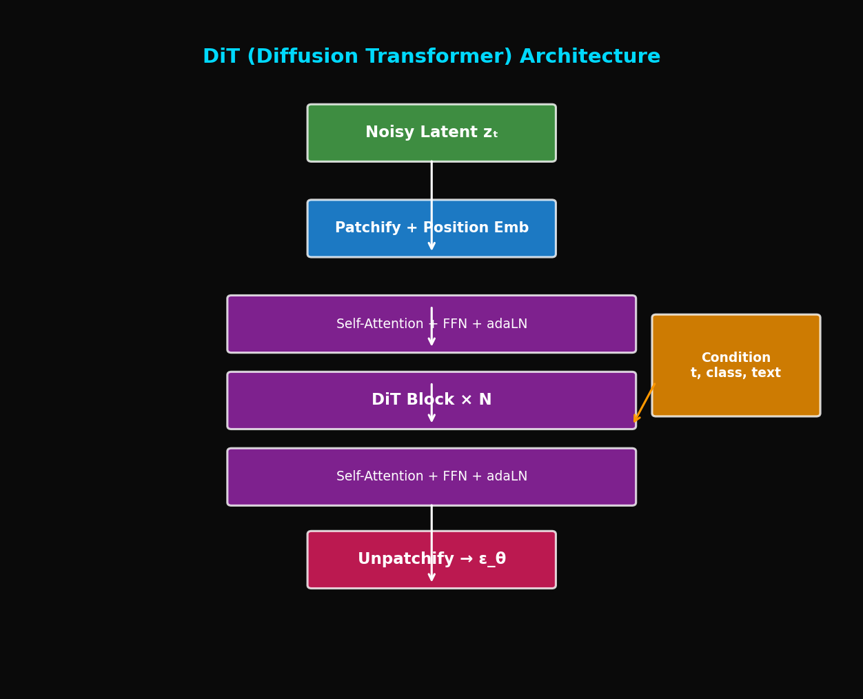
2. DiT Architecture

2.1 Core Idea

"Replace U-Net with Vision Transformer in Diffusion models"

2.2 Input Processing: Patchify

Split image (or latent) into patches:

python

class PatchEmbed(nn.Module):
    def __init__(self, img_size=32, patch_size=2, in_channels=4, embed_dim=768):
        super().__init__()
        self.num_patches = (img_size // patch_size) ** 2
        self.proj = nn.Conv2d(in_channels, embed_dim, patch_size, stride=patch_size)

    def forward(self, x):
        # x: (B, C, H, W) → (B, num_patches, embed_dim)
        x = self.proj(x)  # (B, embed_dim, H', W')
        x = x.flatten(2).transpose(1, 2)  # (B, num_patches, embed_dim)
        return x

Example (Stable Diffusion latent):

Input: 64×64×4 latent
Patch size: 2×2
Number of patches: 32×32 = 1024
Each patch: 2×2×4 = 16 → projected to embed_dim

2.3 Condition Injection: AdaLN

Original U-Net: Add time embedding to ResBlock

DiT: Adaptive Layer Normalization (AdaLN)

$\text{AdaLN}(h, y) = y_s \odot \text{LayerNorm}(h) + y_b$

Where $y_s, y_b$ are scale/shift parameters generated from conditions

python

class AdaLN(nn.Module):
    def __init__(self, hidden_size, condition_dim):
        super().__init__()
        self.norm = nn.LayerNorm(hidden_size, elementwise_affine=False)
        self.adaLN_modulation = nn.Sequential(
            nn.SiLU(),
            nn.Linear(condition_dim, 6 * hidden_size)
        )

    def forward(self, x, c):
        # c: condition (time + class embedding)
        shift_msa, scale_msa, gate_msa, shift_mlp, scale_mlp, gate_mlp = \
            self.adaLN_modulation(c).chunk(6, dim=-1)

        # Used in each block
        return shift_msa, scale_msa, gate_msa, shift_mlp, scale_mlp, gate_mlp

2.4 DiT Block

python

class DiTBlock(nn.Module):
    def __init__(self, hidden_size, num_heads, condition_dim, mlp_ratio=4.0):
        super().__init__()
        self.norm1 = nn.LayerNorm(hidden_size, elementwise_affine=False)
        self.attn = Attention(hidden_size, num_heads)
        self.norm2 = nn.LayerNorm(hidden_size, elementwise_affine=False)
        self.mlp = MLP(hidden_size, int(hidden_size * mlp_ratio))

        # AdaLN modulation
        self.adaLN_modulation = nn.Sequential(
            nn.SiLU(),
            nn.Linear(condition_dim, 6 * hidden_size)
        )

    def forward(self, x, c):
        # c: condition embedding
        shift_msa, scale_msa, gate_msa, shift_mlp, scale_mlp, gate_mlp = \
            self.adaLN_modulation(c).chunk(6, dim=-1)

        # Self-attention with AdaLN
        x_norm = self.norm1(x)
        x_norm = x_norm * (1 + scale_msa.unsqueeze(1)) + shift_msa.unsqueeze(1)
        x = x + gate_msa.unsqueeze(1) * self.attn(x_norm)

        # MLP with AdaLN
        x_norm = self.norm2(x)
        x_norm = x_norm * (1 + scale_mlp.unsqueeze(1)) + shift_mlp.unsqueeze(1)
        x = x + gate_mlp.unsqueeze(1) * self.mlp(x_norm)

        return x

2.5 Output Processing: Unpatchify

Reconstruct patches back to image:

python

class FinalLayer(nn.Module):
    def __init__(self, hidden_size, patch_size, out_channels):
        super().__init__()
        self.norm_final = nn.LayerNorm(hidden_size, elementwise_affine=False)
        self.linear = nn.Linear(hidden_size, patch_size * patch_size * out_channels)
        self.adaLN_modulation = nn.Sequential(
            nn.SiLU(),
            nn.Linear(hidden_size, 2 * hidden_size)
        )

    def forward(self, x, c):
        shift, scale = self.adaLN_modulation(c).chunk(2, dim=-1)
        x = self.norm_final(x) * (1 + scale.unsqueeze(1)) + shift.unsqueeze(1)
        x = self.linear(x)
        return x

def unpatchify(x, patch_size, img_size):
    """
    x: (B, num_patches, patch_size²×C)
    → (B, C, H, W)
    """
    p = patch_size
    h = w = img_size // p
    c = x.shape[-1] // (p * p)

    x = x.reshape(x.shape[0], h, w, p, p, c)
    x = torch.einsum('nhwpqc->nchpwq', x)
    x = x.reshape(x.shape[0], c, h * p, w * p)
    return x

3. Complete DiT Model

3.1 Model Definition

python

class DiT(nn.Module):
    def __init__(
        self,
        input_size=32,          # Latent size
        patch_size=2,
        in_channels=4,
        hidden_size=1152,
        depth=28,
        num_heads=16,
        mlp_ratio=4.0,
        num_classes=1000,       # For class conditioning
        learn_sigma=True,
    ):
        super().__init__()
        self.in_channels = in_channels
        self.out_channels = in_channels * 2 if learn_sigma else in_channels
        self.patch_size = patch_size
        self.num_heads = num_heads

        # Patch embedding
        self.x_embedder = PatchEmbed(input_size, patch_size, in_channels, hidden_size)
        num_patches = self.x_embedder.num_patches

        # Time embedding
        self.t_embedder = TimestepEmbedder(hidden_size)

        # Class embedding
        self.y_embedder = LabelEmbedder(num_classes, hidden_size)

        # Positional embedding
        self.pos_embed = nn.Parameter(torch.zeros(1, num_patches, hidden_size))

        # DiT blocks
        self.blocks = nn.ModuleList([
            DiTBlock(hidden_size, num_heads, hidden_size, mlp_ratio)
            for _ in range(depth)
        ])

        # Final layer
        self.final_layer = FinalLayer(hidden_size, patch_size, self.out_channels)

        self.initialize_weights()

    def forward(self, x, t, y):
        """
        x: (B, C, H, W) noisy latent
        t: (B,) timesteps
        y: (B,) class labels
        """
        # Patchify + positional embedding
        x = self.x_embedder(x) + self.pos_embed

        # Condition embedding
        t = self.t_embedder(t)
        y = self.y_embedder(y)
        c = t + y  # Combined condition

        # DiT blocks
        for block in self.blocks:
            x = block(x, c)

        # Final layer
        x = self.final_layer(x, c)

        # Unpatchify
        x = unpatchify(x, self.patch_size, self.input_size)

        return x

3.2 Model Variants

Model	Layers	Hidden Size	Heads	Parameters
DiT-S	12	384	6	33M
DiT-B	12	768	12	130M
DiT-L	24	1024	16	458M
DiT-XL	28	1152	16	675M

4. Scaling Law Analysis

4.1 Model Size vs Performance

Key finding from DiT paper:

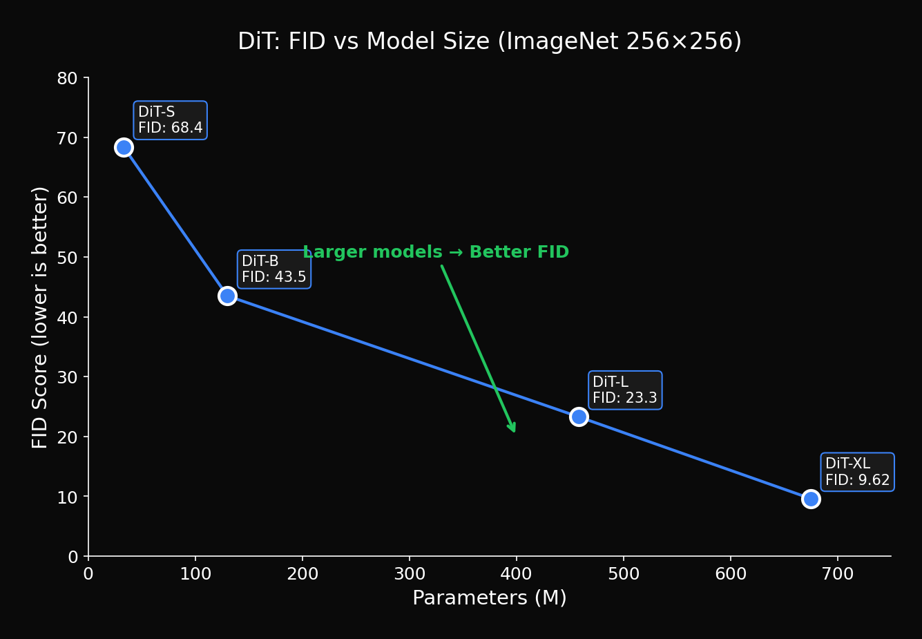
DiT: FID vs Model Size (ImageNet 256×256)

Consistent improvement: FID decreases steadily with parameter increase

4.2 Compute vs Performance

Compute (GFLOPs)	DiT FID	U-Net FID
50	43.5	52.3
100	25.1	31.8
200	12.4	18.6
500	4.9	9.3

DiT is more efficient at the same compute

4.3 Scaling Law Formula

Empirically discovered relationship:

$\text{FID} \approx A \cdot C^{-\alpha}$

Where:

$C$ : Compute (GFLOPs)
$\alpha \approx 0.4$ for DiT
$\alpha \approx 0.25$ for U-Net

DiT has larger scaling exponent → More favorable for scaling

5. Training and Sampling

5.1 Training Code

python

def train_step(model, vae, x, y, noise_scheduler):
    # 1. Encode to latent
    with torch.no_grad():
        z = vae.encode(x).latent_dist.sample() * 0.18215

    # 2. Sample timestep
    t = torch.randint(0, noise_scheduler.num_train_timesteps, (z.shape[0],))

    # 3. Add noise
    noise = torch.randn_like(z)
    z_t = noise_scheduler.add_noise(z, noise, t)

    # 4. Predict noise (or v-prediction)
    model_output = model(z_t, t, y)

    # 5. Compute loss
    if model.learn_sigma:
        noise_pred, _ = model_output.chunk(2, dim=1)
    else:
        noise_pred = model_output

    loss = F.mse_loss(noise_pred, noise)

    return loss

5.2 Classifier-Free Guidance

python

@torch.no_grad()
def sample(model, vae, num_samples, num_classes, cfg_scale=4.0, num_steps=250):
    # Random class labels
    y = torch.randint(0, num_classes, (num_samples,))
    y_null = torch.full_like(y, num_classes)  # Null class

    # Initial noise
    z = torch.randn(num_samples, 4, 32, 32)

    # Sampling loop
    for t in tqdm(reversed(range(num_steps))):
        t_batch = torch.full((num_samples,), t)

        # CFG: predict both conditional and unconditional
        z_input = torch.cat([z, z], dim=0)
        t_input = torch.cat([t_batch, t_batch], dim=0)
        y_input = torch.cat([y, y_null], dim=0)

        model_output = model(z_input, t_input, y_input)
        eps_cond, eps_uncond = model_output.chunk(2, dim=0)

        # Guidance
        eps = eps_uncond + cfg_scale * (eps_cond - eps_uncond)

        # DDPM step
        z = ddpm_step(z, eps, t)

    # Decode
    z = z / 0.18215
    images = vae.decode(z).sample

    return images

6. Applications of DiT

6.1 Sora (OpenAI)

Sora extends DiT to video generation:

Video DiT:
- Input: 3D latent (T × H × W × C)
- Patchify: Spacetime patches
- Attention: Spatial + Temporal
- Output: Video frames

Key Changes:

2D patches → 3D patches
2D positional encoding → 3D positional encoding
Added cross-frame attention

6.2 Flux (Black Forest Labs)

Flux optimizes DiT for T2I:

MMDiT (Multimodal DiT): Text-image joint attention
Rectified Flow: Faster sampling
Larger Scale: 12B parameters

6.3 PixArt Series

PixArt-α, PixArt-Σ:

Efficient training (10% cost)
Uses T5 text encoder
Class-to-text transfer learning

7. Implementation Optimization

7.1 Flash Attention

python

from flash_attn import flash_attn_func

class FlashAttention(nn.Module):
    def __init__(self, dim, num_heads):
        super().__init__()
        self.num_heads = num_heads
        self.head_dim = dim // num_heads
        self.qkv = nn.Linear(dim, dim * 3)
        self.proj = nn.Linear(dim, dim)

    def forward(self, x):
        B, N, C = x.shape
        qkv = self.qkv(x).reshape(B, N, 3, self.num_heads, self.head_dim)
        q, k, v = qkv.unbind(2)

        # Flash Attention
        out = flash_attn_func(q, k, v)

        out = out.reshape(B, N, C)
        return self.proj(out)

7.2 Gradient Checkpointing

python

class DiTWithCheckpoint(DiT):
    def forward(self, x, t, y):
        x = self.x_embedder(x) + self.pos_embed
        c = self.t_embedder(t) + self.y_embedder(y)

        # Gradient checkpointing for memory efficiency
        for block in self.blocks:
            x = checkpoint(block, x, c, use_reentrant=False)

        x = self.final_layer(x, c)
        return unpatchify(x, self.patch_size, self.input_size)

7.3 Mixed Precision Training

python

from torch.cuda.amp import autocast, GradScaler

scaler = GradScaler()

for batch in dataloader:
    with autocast():
        loss = train_step(model, vae, batch['image'], batch['label'])

    scaler.scale(loss).backward()
    scaler.step(optimizer)
    scaler.update()

8. Experimental Results

8.1 ImageNet 256×256

Model	FID ↓	IS ↑	Parameters
ADM	10.94	100.98	554M
LDM-4	10.56	103.49	400M
DiT-XL/2	2.27	278.24	675M

DiT-XL achieves SOTA!

8.2 ImageNet 512×512

Model	FID ↓	Parameters
ADM-G	7.72	608M
DiT-XL/2	3.04	675M

8.3 Scaling Experiments

Model	GFLOPs	FID
DiT-S/2	6	68.4
DiT-B/2	23	43.5
DiT-L/2	80	23.3
DiT-XL/2	119	9.6
DiT-XL/2 (longer training)	119	2.27

9. Conclusion

DiT opened a new era for Diffusion models:

Scalable Architecture: Leverages Transformer's scaling laws
Consistent Performance Improvement: Quality proportional to size
Versatility: Supports various modalities including image, video, 3D
Efficiency: Better performance at the same compute

This is why the latest generative models like Sora and Flux are based on DiT.

In the next article, we'll cover PixArt-α: efficient DiT training methods and the use of T5 text encoder.

References

Peebles, W., & Xie, S. (2023). Scalable Diffusion Models with Transformers. ICCV 2023
Dosovitskiy, A., et al. (2021). An Image is Worth 16x16 Words: Transformers for Image Recognition at Scale. ICLR 2021
Chen, J., et al. (2023). PixArt-α: Fast Training of Diffusion Transformer for Photorealistic Text-to-Image Synthesis. arXiv
Esser, P., et al. (2024). Scaling Rectified Flow Transformers for High-Resolution Image Synthesis. arXiv

Tags: #DiT #Diffusion-Transformer #Scaling-Law #Sora #Vision-Transformer #Image-Generation

The complete code for this article is available in the attached Jupyter Notebook.